Setting up

Let’s set up and get our hands dirty.

library(cmdstanr)
library(brms)
library(tidyverse)
library(knitr)
library(patchwork)
library(bayesplot)

source("RTmixture.R")

ggplot2::theme_set(cowplot::theme_cowplot())
options(mc.cores = parallel::detectCores(), brms.backend = "cmdstanr")

cache_dir <- "_RTmixture_cache"
if(!dir.exists(cache_dir)) {
  dir.create(cache_dir)
}

First, we’ll generate some fake data to test the model against. Below is just a more concise and optimized version of the random generation scheme I showed earlier.

rRTmixture <- function(n, meanlog, sdlog, mix, shift, upper) { 
  ifelse(runif(n) < mix,  
         runif(n, 0, upper),  
         shift + rlnorm(n, meanlog = meanlog, sdlog = sdlog)) 
} 
 

Then let us generate some data

set.seed(31546522)
# Bounds of the data
max_shift <- 0.3
shift <- runif(1) * max_shift
upper <- 10
mix <- 0.1

N <- 100
Intercept <- 0.3
beta <- 0.5
X <- rnorm(N)
mu <- rep(Intercept, N) + beta * X
sigma <- 0.5

rt <- rRTmixture(N, meanlog = mu, sdlog = sigma, mix = mix, shift = shift, upper = upper)

dd <- data.frame(rt = rt, x = X, max_shift = max_shift, upper = upper)

Looking nice!

ggplot(dd, aes(x = rt)) + geom_density()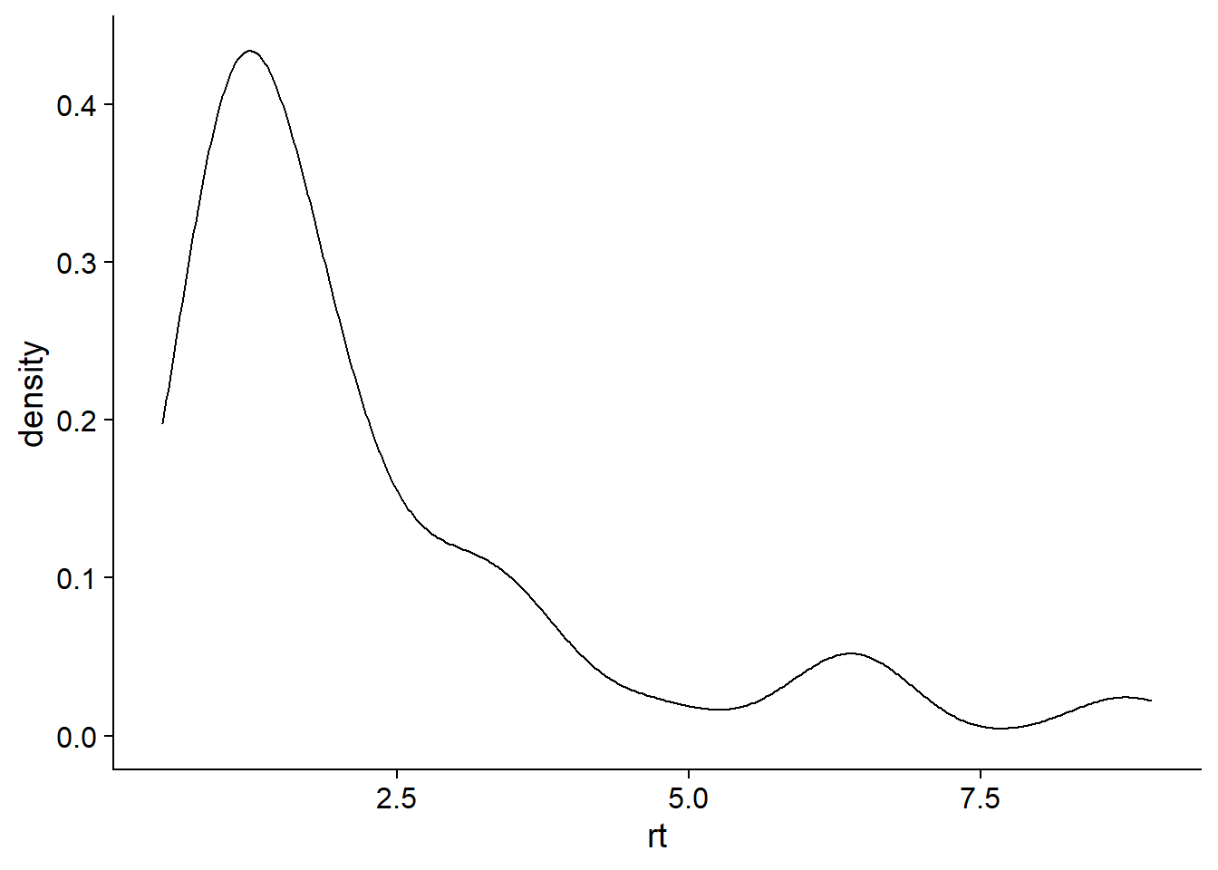

Core of the family

Now we need the Stan implementation of the family. That is probably the most technical part. Stan user’s guide has some background on mixture models in Stan. We’ll note that times before shift can only come from the uniform component and times after upper can only come from the lognormal component. For others we mix both a lognormal and the uniform via log_mix.

With the Stan code ready, we then define the parameters of the distribution in a way that brms understands.

stan_funs_base <- stanvar(block = "functions", scode = " 
  real RTmixture_lpdf(real y, real mu, real sigma, real mix,  
                      real shiftprop, real max_shift, real upper) { 
    real shift = shiftprop * max_shift; 
    if(y <= shift) { 
      // Could only be created by the contamination 
      return log(mix) + uniform_lpdf(y | 0, upper); 
    } else if(y >= upper) { 
      // Could only come from the lognormal 
      return log1m(mix) + lognormal_lpdf(y - shift | mu, sigma); 
    } else { 
      // Actually mixing 
      real lognormal_llh = lognormal_lpdf(y - shift | mu, sigma); 
      real uniform_llh = uniform_lpdf(y | 0, upper); 
      return log_mix(mix, uniform_llh, lognormal_llh); 
    } 
  } 
 
") 
 
 
 
RTmixture <- custom_family( 
  "RTmixture",  
  dpars = c("mu", "sigma", "mix", "shiftprop"), # Those will be estimated 
  links = c("identity", "log", "logit", "logit"), 
  type = "real", 
  lb = c(NA, 0, 0, 0), # bounds for the parameters  
  ub = c(NA, NA, 1, 1), 
  vars = c("vreal1[n]", "vreal2[n]") # Data for max_shift and upper (known) 
) 

And we are ready to fit! We will put a weakly informative beta(1,5) prior on the proportion of contamination - this means we a prior believe that there is a 95% chance that the contamination is lower than qbeta(0.95, 1, 5) = 0.4507197. One could definitely be justified in tightening this prior even further toward zero for many tasks. vreal is just brms’s way of annotating arbitrary additional data for the distribution. We need to pass both the family and the associated stanvars.

fit_mix <- brm(rt | vreal(max_shift, upper) ~ x, data = dd, family = RTmixture, 
               stanvars = stan_funs_base, 
               refresh = 0,
               file = paste0(cache_dir, "/mix"), file_refit = "on_change",
               prior = c(prior(beta(1, 5), class = "mix")))
fit_mix

##  Family: RTmixture 
##   Links: mu = identity; sigma = identity; mix = identity; shiftprop = identity 
## Formula: rt | vreal(max_shift, upper) ~ x 
##    Data: dd (Number of observations: 100) 
##   Draws: 4 chains, each with iter = 1000; warmup = 0; thin = 1;
##          total post-warmup draws = 4000
## 
## Population-Level Effects: 
##           Estimate Est.Error l-95% CI u-95% CI Rhat Bulk_ESS Tail_ESS
## Intercept     0.33      0.07     0.20     0.48 1.00     2097     2242
## x             0.44      0.05     0.33     0.54 1.00     2368     2460
## 
## Family Specific Parameters: 
##           Estimate Est.Error l-95% CI u-95% CI Rhat Bulk_ESS Tail_ESS
## sigma         0.45      0.05     0.36     0.56 1.00     2379     1976
## mix           0.13      0.05     0.05     0.24 1.00     3159     2589
## shiftprop     0.82      0.18     0.32     1.00 1.00     1640     1623
## 
## Draws were sampled using sample(hmc). For each parameter, Bulk_ESS
## and Tail_ESS are effective sample size measures, and Rhat is the potential
## scale reduction factor on split chains (at convergence, Rhat = 1).

We note that we have quite good recovery of the effect of x (simulated as 0.5) and of sigma (which was 0.5), but 100 observations are not enough to constrain the mix parameter really well (simulated as 0.1).

For comparison, we also fit the default shifted lognormal as implemented in brms.

fit_base <- brm(rt ~ x, data = dd, family = shifted_lognormal, refresh = 0,
                file = paste0(cache_dir, "/base"), file_refit = "on_change")

fit_base

##  Family: shifted_lognormal 
##   Links: mu = identity; sigma = identity; ndt = identity 
## Formula: rt ~ x 
##    Data: dd (Number of observations: 100) 
##   Draws: 4 chains, each with iter = 1000; warmup = 0; thin = 1;
##          total post-warmup draws = 4000
## 
## Population-Level Effects: 
##           Estimate Est.Error l-95% CI u-95% CI Rhat Bulk_ESS Tail_ESS
## Intercept     0.34      0.09     0.16     0.53 1.00     1958     1949
## x             0.47      0.07     0.33     0.61 1.00     2711     2495
## 
## Family Specific Parameters: 
##       Estimate Est.Error l-95% CI u-95% CI Rhat Bulk_ESS Tail_ESS
## sigma     0.69      0.07     0.56     0.82 1.00     1883     1802
## ndt       0.34      0.07     0.17     0.44 1.00     1634     1420
## 
## Draws were sampled using sample(hmc). For each parameter, Bulk_ESS
## and Tail_ESS are effective sample size measures, and Rhat is the potential
## scale reduction factor on split chains (at convergence, Rhat = 1).

We see that the inferences for sigma are a bit biased but this is not necessarily only due to the mixture, another potentially biasing is the different handling of the shift.

Censoring + constant shift

To support censoring in brms the family has to come with log CDF (cumulative distribution function) and log CCDF (complementary CDF) implementations in Stan, which we provide below. Those match the _lpdf pretty closely.

 
stan_funs <- stan_funs_base + stanvar(block = "functions", scode = " 
  real RTmixture_lcdf(real y, real mu, real sigma, real mix,  
                      real shiftprop, real max_shift, real upper) { 
    real shift = shiftprop * max_shift; 
    if(y <= shift) { 
      return log(mix) + uniform_lcdf(y | 0, upper); 
    } else if(y >= upper) { 
      // The whole uniform part is below, so the mixture part is log(1) = 0 
      return log_mix(mix, 0, lognormal_lcdf(y - shift | mu, sigma)); 
    } else { 
      real lognormal_llh = lognormal_lcdf(y - shift | mu, sigma); 
      real uniform_llh = uniform_lcdf(y | 0, upper); 
      return log_mix(mix, uniform_llh, lognormal_llh); 
    } 
  } 
   
  real RTmixture_lccdf(real y, real mu, real sigma, real mix,  
                      real shiftprop, real max_shift, real upper) { 
 
    real shift = shiftprop * max_shift; 
    if(y <= shift) { 
      // The whole lognormal part is above, so the mixture part is log(1) = 0 
      return log_mix(mix, uniform_lccdf(y | 0, upper), 0); 
    } else if(y >= upper) { 
      return log1m(mix) + lognormal_lccdf(y - shift | mu, sigma); 
    } else { 
      real lognormal_llh = lognormal_lccdf(y - shift | mu, sigma); 
      real uniform_llh = uniform_lccdf(y | 0, upper); 
      return log_mix(mix, uniform_llh, lognormal_llh); 
    } 
 
  } 
") 
 

To test if this work, we’ll do quite aggressive censoring and treat anything larger than 1.5 as censored. In most cases it makes sense to have upper be the same as the censoring bound, so we’ll do that

set.seed(25462255)
shift <- 0.15
cens_bound <- upper <- 1.5
mix <- 0.08

N <- 110
Intercept <- 0.5
beta <- -0.3
X <- rnorm(N)
mu <- rep(Intercept, N) + beta * X
sigma <- 0.4

rt <- rRTmixture(N, meanlog = mu, sdlog = sigma, 
                 mix = mix, shift = shift, upper = upper)
censored <- rt > cens_bound
rt[censored] <- cens_bound

dd_cens <- data.frame(rt = rt, 
                      censored = if_else(censored, "right", "none"),  
                      x = X, max_shift = shift, upper = upper)

Finally, this model starts to be problematic if we try to estimate shift (well, actually shiftprop) as well. An easy way to to make shift always equal to max_shift is to set a constant prior on shiftprop, as we do below.

fit_mix_cens <- brm(rt | vreal(max_shift, upper) + cens(censored) ~ x, 
                    data = dd_cens, 
                    family = RTmixture, 
                    stanvars = stan_funs, 
                    refresh = 0,
                    file = paste0(cache_dir, "/mix_cens"), 
                    file_refit = "on_change",
                    prior = c(prior(beta(1, 5), class = "mix"),
                              prior(constant(1), class = "shiftprop")))
fit_mix_cens

##  Family: RTmixture 
##   Links: mu = identity; sigma = identity; mix = identity; shiftprop = identity 
## Formula: rt | vreal(max_shift, upper) + cens(censored) ~ x 
##    Data: dd_cens (Number of observations: 110) 
##   Draws: 4 chains, each with iter = 1000; warmup = 0; thin = 1;
##          total post-warmup draws = 4000
## 
## Population-Level Effects: 
##           Estimate Est.Error l-95% CI u-95% CI Rhat Bulk_ESS Tail_ESS
## Intercept     0.46      0.08     0.34     0.65 1.00     2022     1674
## x            -0.23      0.07    -0.38    -0.12 1.00     2094     1606
## 
## Family Specific Parameters: 
##           Estimate Est.Error l-95% CI u-95% CI Rhat Bulk_ESS Tail_ESS
## sigma         0.36      0.07     0.26     0.53 1.00     2019     2565
## mix           0.15      0.05     0.07     0.25 1.00     2943     2595
## shiftprop     1.00      0.00     1.00     1.00   NA       NA       NA
## 
## Draws were sampled using sample(hmc). For each parameter, Bulk_ESS
## and Tail_ESS are effective sample size measures, and Rhat is the potential
## scale reduction factor on split chains (at convergence, Rhat = 1).

It works and the inferences are reasonably close to what we simulated with. A more thorough evaluation would require simulation-based calibration, which would be nice, but would require a bit more energy than I have now. But it seems that at least the models are not completely wrong.

If you want to model varying shift but having issues fitting, it might make sense to adjust max_shift on a per-group basis to have max_shift larger only than a small proportion of observations in this group. As noted above, if you set different max_shift per for example subject_id, you should also have shiftprop ~ subject_id or the model might not make sense.

Making predictions

We successfully fitted a few models, but there are some tweaks we need to do to make full use of the family. We might for example want to make predictions - e.g. to make posterior predictive checks - so we also need to implement prediction code. You’ll notice that we are just extracting the parameters from the prepared predictions and passing those to the generator function we defined earlier.

 
posterior_predict_RTmixture <- function(i, prep, ...) { 
  if((!is.null(prep$data$lb) && prep$data$lb[i] > 0) ||  
     (!is.null(prep$data$ub) && prep$data$ub[i] < Inf)) { 
    stop("Predictions for truncated distributions not supported") 
  }   
   
  mu <- brms:::get_dpar(prep, "mu", i = i) 
  sigma <- brms:::get_dpar(prep, "sigma", i = i) 
  mix <- brms:::get_dpar(prep, "mix", i = i) 
  shiftprop <- brms:::get_dpar(prep, "shiftprop", i = i) 
   
  max_shift <- prep$data$vreal1[i] 
  upper <- prep$data$vreal2[i] 
  shift = shiftprop * max_shift 
   
  rRTmixture(prep$ndraws, meanlog = mu, sdlog = sigma,  
             mix = mix, shift = shift, upper = upper) 
} 
 

Note that the get_dpar helper that simplifies some bookeeping is currently internal in brms, but will be exposed in upcoming release.

With that, we can do a posterior predictive check for both models. We use only single core for predictions, because on Windows, multicore is slow and will not be able to access the custom prediction functions.

pp_mix <- pp_check(fit_mix, type = "dens_overlay", ndraws = 100,  cores = 1)  +
  ggtitle("Mixture")
pp_base <- pp_check(fit_base, type = "dens_overlay", ndraws = 100,  cores = 1) +
  ggtitle("Shifted lognormal")
pp_mix / pp_base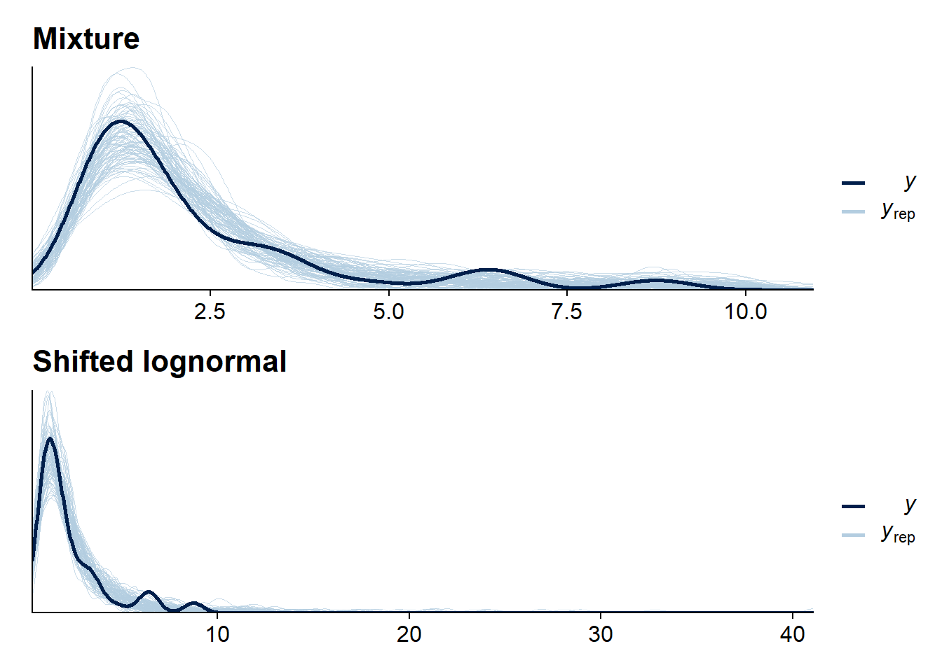

For this dataset, the mixture is not doing that much in improving the bulk of the predictions, but it manages to avoid the very long tail the lognormal-only model needs to accomodate the larger values.

We might also look at checks of the censored model. brms does not directly support predicting censored variables (because the data passed to the model are not enough to completely determine all censoring), but we can easily do this manually:

set.seed(123566)
pred_cens <- posterior_predict(fit_mix_cens, cores = 1)
pred_cens_cens <- pred_cens
# Do the censoring
pred_cens_cens[pred_cens > cens_bound] <- cens_bound 
samples_dens <- sample(1:(dim(pred_cens)[1]), size = 50)
ppc_cens1 <- ppc_dens_overlay(dd_cens$rt, pred_cens_cens[samples_dens,])  + 
  ggtitle("Censored dataset")
ppc_cens2 <- ppc_stat(1.0 * (dd_cens$censored == "right"), 
                      1.0 * (pred_cens >= cens_bound), 
                      binwidth = 0.02) + 
  ggtitle("Proportion censored")

ppc_cens1 + ppc_cens2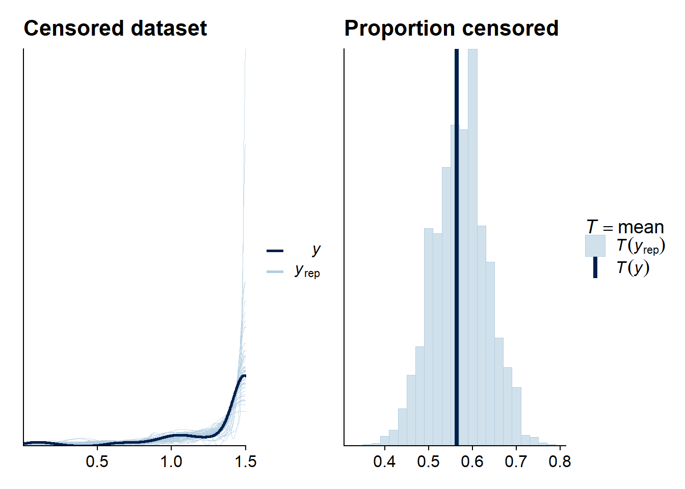

The model seems to do OK.

Using loo

Similarly, we might want to do model comparison or stacking with loo, so we also implement the log_lik function.

## Needed for numerical stability 
## from http://tr.im/hH5A 
logsumexp <- function (x) { 
  y = max(x) 
  y + log(sum(exp(x - y))) 
} 
 
 
RTmixture_lpdf <- function(y, meanlog, sdlog, mix, shift, upper) { 
  unif_llh = dunif(y , min = 0, max = upper, log = TRUE) 
  lognormal_llh = dlnorm(y - shift, meanlog = meanlog, sdlog = sdlog, log = TRUE) -  
    plnorm(upper - shift, meanlog = meanlog, sdlog = sdlog, log.p = TRUE) 
   
   
  # Computing logsumexp(log(mix) + unif_llh, log1p(-mix) + lognormal_llh)     
  # but vectorized 
  llh_matrix <- array(NA_real_, dim = c(2, max(length(unif_llh), length(lognormal_llh)))) 
  llh_matrix[1,] <- log(mix) + unif_llh 
  llh_matrix[2,] <- log1p(-mix) + lognormal_llh 
  apply(llh_matrix, MARGIN = 2, FUN = logsumexp) 
} 
 
log_lik_RTmixture <- function(i, draws) { 
  mu <- brms:::get_dpar(draws, "mu", i = i) 
  sigma <- brms:::get_dpar(draws, "sigma", i = i) 
  mix <- brms:::get_dpar(draws, "mix", i = i) 
  shiftprop <- brms:::get_dpar(draws, "shiftprop", i = i) 
   
  max_shift <- draws$data$vreal1[i] 
  upper <- draws$data$vreal2[i] 
  shift = shiftprop * max_shift 
   
  y <- draws$data$Y[i] 
  RTmixture_lpdf(y, meanlog = mu, sdlog = sigma,  
                 mix = mix, shift = shift, upper = upper) 
   
} 

And now, we can compare the models:

fit_mix <- add_criterion(fit_mix, "loo", cores = 1)
fit_base <- add_criterion(fit_base, "loo", cores = 1)
loo_compare(fit_mix, fit_base)

##          elpd_diff se_diff
## fit_mix   0.0       0.0   
## fit_base -7.5       5.3

No surprise here - we simulated the data with the mixture model and indeed, this is preferred to a different model. Also, the shifted-lognormal model has one very influential observation, which turns out to be the smallest observed reaction time.

dd$rt[fit_base$criteria$loo$diagnostics$pareto_k > 0.7]

## [1] 0.4909057

min(dd$rt)

## [1] 0.4909057

This once again shows that the lognormal has problem accomodating both the high and low contamination (while it is plausible it could accomodate a small amount of just high or just low contamination quite well).

Crazy models

Since brms is great, we can now do all sorts of stuff like put predictors on the mix parameter - e.g. to get a per-subject estimate of the amount of contamination.

To do this, we’ll also put a weakly informative prior on the intercept for the mixture that assumes low contamination and we don’t expect huge variability in the amount of contamination (with wider priors the model starts to diverge as we would need much more data to constrain it well).

set.seed(35486622)
dd_subj <- dd_cens
dd_subj$subject_id <- sample(1:12, size = nrow(dd_cens), replace = TRUE)

fit_mix_all <- brm(
  bf(rt | vreal(max_shift, upper) + cens(censored) ~ x, 
     mix ~ 1 + (1 | subject_id),
     family = RTmixture),
  data = dd_subj,
  stanvars = stan_funs, 
               refresh = 0,
               file = paste0(cache_dir, "/mix_all"), file_refit = "on_change",
               prior = c(prior(normal(-3, 1), class = "Intercept", dpar = "mix"),
                         prior(normal(0,0.5), class = "sd", dpar = "mix"),
                         prior(constant(1), class = "shiftprop")))

fit_mix_all

##  Family: RTmixture 
##   Links: mu = identity; sigma = identity; mix = logit; shiftprop = identity 
## Formula: rt | vreal(max_shift, upper) + cens(censored) ~ x 
##          mix ~ 1 + (1 | subject_id)
##    Data: dd_subj (Number of observations: 110) 
##   Draws: 4 chains, each with iter = 1000; warmup = 0; thin = 1;
##          total post-warmup draws = 4000
## 
## Group-Level Effects: 
## ~subject_id (Number of levels: 12) 
##                   Estimate Est.Error l-95% CI u-95% CI Rhat Bulk_ESS Tail_ESS
## sd(mix_Intercept)     0.38      0.29     0.02     1.07 1.00     2706     2137
## 
## Population-Level Effects: 
##               Estimate Est.Error l-95% CI u-95% CI Rhat Bulk_ESS Tail_ESS
## Intercept         0.45      0.07     0.33     0.62 1.00     3586     2305
## mix_Intercept    -2.05      0.44    -2.96    -1.25 1.00     4207     2807
## x                -0.22      0.06    -0.37    -0.11 1.00     3715     2666
## 
## Family Specific Parameters: 
##           Estimate Est.Error l-95% CI u-95% CI Rhat Bulk_ESS Tail_ESS
## sigma         0.37      0.07     0.26     0.54 1.00     3534     3025
## shiftprop     1.00      0.00     1.00     1.00   NA       NA       NA
## 
## Draws were sampled using sample(hmc). For each parameter, Bulk_ESS
## and Tail_ESS are effective sample size measures, and Rhat is the potential
## scale reduction factor on split chains (at convergence, Rhat = 1).

Checking that posterior predictions work:

set.seed(1233354)
pred_cens <- posterior_predict(fit_mix_all, cores = 1)
pred_cens_cens <- pred_cens
pred_cens_cens[pred_cens > cens_bound] <- cens_bound 
samples_dens <- sample(1:(dim(pred_cens)[1]), size = 50)
ppc_dens_overlay(dd_cens$rt, pred_cens_cens[samples_dens,])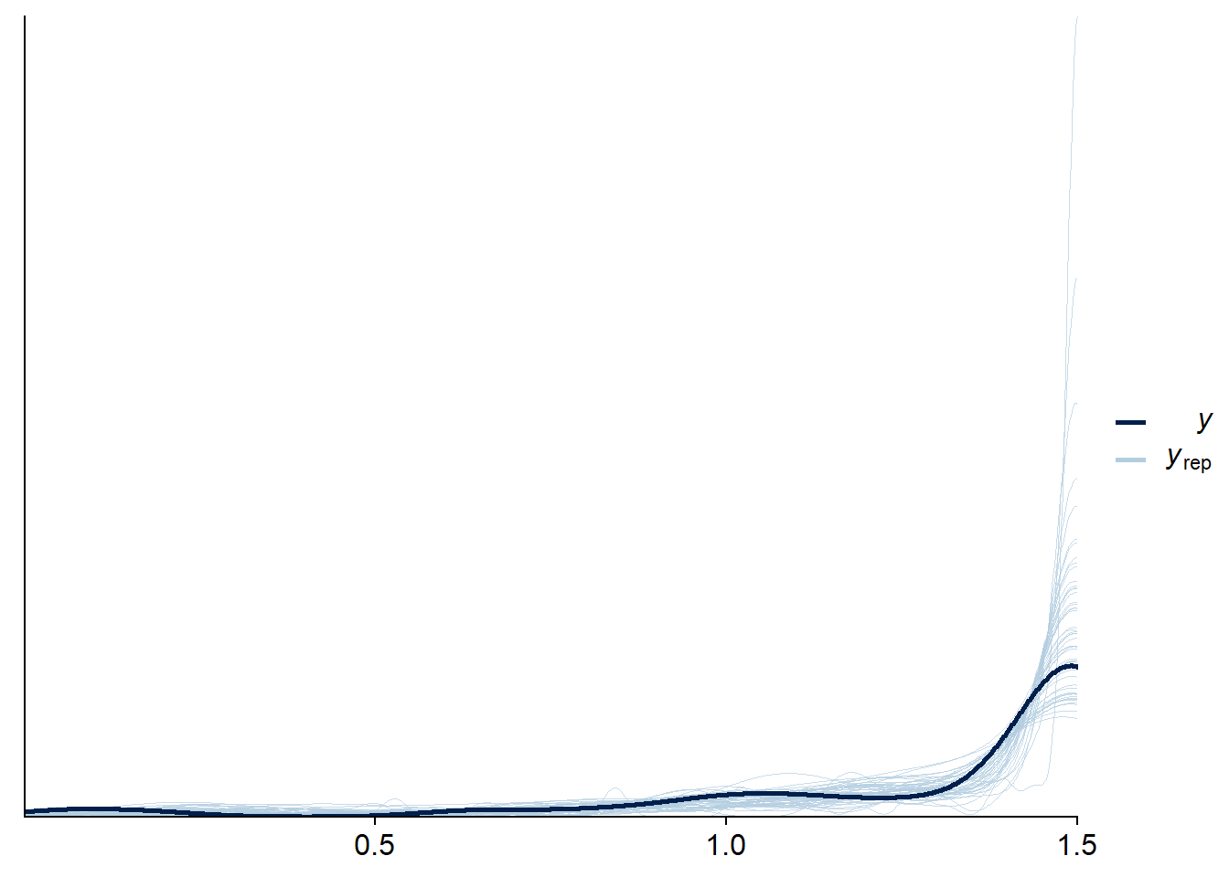

We can also do multivariate models where some of the predictors are correlated across answers:

set.seed(0245562)
# Build a dataset containing two separate predictions
dd_both <- dd
dd_both$rt2 <- dd_cens$rt[1:nrow(dd_both)]
dd_both$x2 <- dd_cens$x[1:nrow(dd_both)]
dd_both$censored2 <- dd_cens$censored[1:nrow(dd_both)]
dd_both$max_shift2 <- dd_cens$max_shift[1:nrow(dd_both)]
dd_both$upper2 <- dd_cens$upper[1:nrow(dd_both)]
dd_both$subject_id <- sample(1:12, size = nrow(dd_both), replace = TRUE)

fit_mix_multivar <- brm(
  bf(rt | vreal(max_shift, upper)  ~ x, 
     mix ~ 1 + (1 | p | subject_id),
     family = RTmixture) +
  bf(rt2 | vreal(max_shift2, upper2) + cens(censored2) ~ x2, 
   mix ~ 1 + (1 | p | subject_id),
     family = RTmixture),
  data = dd_both,
  stanvars = stan_funs, 
  refresh = 0,
  file = paste0(cache_dir, "/mix_multivar"), file_refit = "on_change",
  prior = c(prior(normal(-3, 1), class = "Intercept", dpar = "mix", resp = "rt"),
           prior(normal(0,0.5), class = "sd", dpar = "mix", resp = "rt"),
           prior(constant(1), class = "shiftprop", resp = "rt"),
           prior(normal(-3, 1), class = "Intercept", dpar = "mix", resp = "rt2"),
           prior(normal(0,0.5), class = "sd", dpar = "mix", resp = "rt2"),
           prior(constant(1), class = "shiftprop", resp = "rt2")
           ),
  adapt_delta = 0.95
  )

## Setting 'rescor' to FALSE by default for this model

fit_mix_multivar

##  Family: MV(RTmixture, RTmixture) 
##   Links: mu = identity; sigma = identity; mix = logit; shiftprop = identity
##          mu = identity; sigma = identity; mix = logit; shiftprop = identity 
## Formula: rt | vreal(max_shift, upper) ~ x 
##          mix ~ 1 + (1 | p | subject_id)
##          rt2 | vreal(max_shift2, upper2) + cens(censored2) ~ x2 
##          mix ~ 1 + (1 | p | subject_id)
##    Data: dd_both (Number of observations: 100) 
##   Draws: 4 chains, each with iter = 1000; warmup = 0; thin = 1;
##          total post-warmup draws = 4000
## 
## Group-Level Effects: 
## ~subject_id (Number of levels: 12) 
##                                         Estimate Est.Error l-95% CI u-95% CI
## sd(mix_rt_Intercept)                        0.33      0.25     0.01     0.91
## sd(mix_rt2_Intercept)                       0.37      0.27     0.02     1.01
## cor(mix_rt_Intercept,mix_rt2_Intercept)     0.00      0.58    -0.95     0.95
##                                         Rhat Bulk_ESS Tail_ESS
## sd(mix_rt_Intercept)                    1.00     2713     1787
## sd(mix_rt2_Intercept)                   1.00     2587     2046
## cor(mix_rt_Intercept,mix_rt2_Intercept) 1.00     4331     2836
## 
## Population-Level Effects: 
##                   Estimate Est.Error l-95% CI u-95% CI Rhat Bulk_ESS Tail_ESS
## rt_Intercept          0.30      0.06     0.18     0.43 1.00     4743     3085
## mix_rt_Intercept     -2.28      0.54    -3.50    -1.35 1.00     4035     1843
## rt2_Intercept         0.43      0.08     0.31     0.60 1.00     3258     1826
## mix_rt2_Intercept    -1.91      0.44    -2.80    -1.11 1.00     4456     3016
## rt_x                  0.46      0.05     0.36     0.56 1.00     5440     2978
## rt2_x2               -0.25      0.07    -0.40    -0.13 1.00     3316     2106
## 
## Family Specific Parameters: 
##               Estimate Est.Error l-95% CI u-95% CI Rhat Bulk_ESS Tail_ESS
## sigma_rt          0.49      0.05     0.40     0.60 1.00     4907     3014
## sigma_rt2         0.36      0.07     0.25     0.53 1.00     3449     2885
## shiftprop_rt      1.00      0.00     1.00     1.00   NA       NA       NA
## shiftprop_rt2     1.00      0.00     1.00     1.00   NA       NA       NA
## 
## Draws were sampled using sample(hmc). For each parameter, Bulk_ESS
## and Tail_ESS are effective sample size measures, and Rhat is the potential
## scale reduction factor on split chains (at convergence, Rhat = 1).

Testing that predictions work even for multivariate models. Note that we don’t bother with censoring for rt2 so the predictions look wrong.

pp_check(fit_mix_multivar, resp = "rt", ndraws = 30, cores = 1)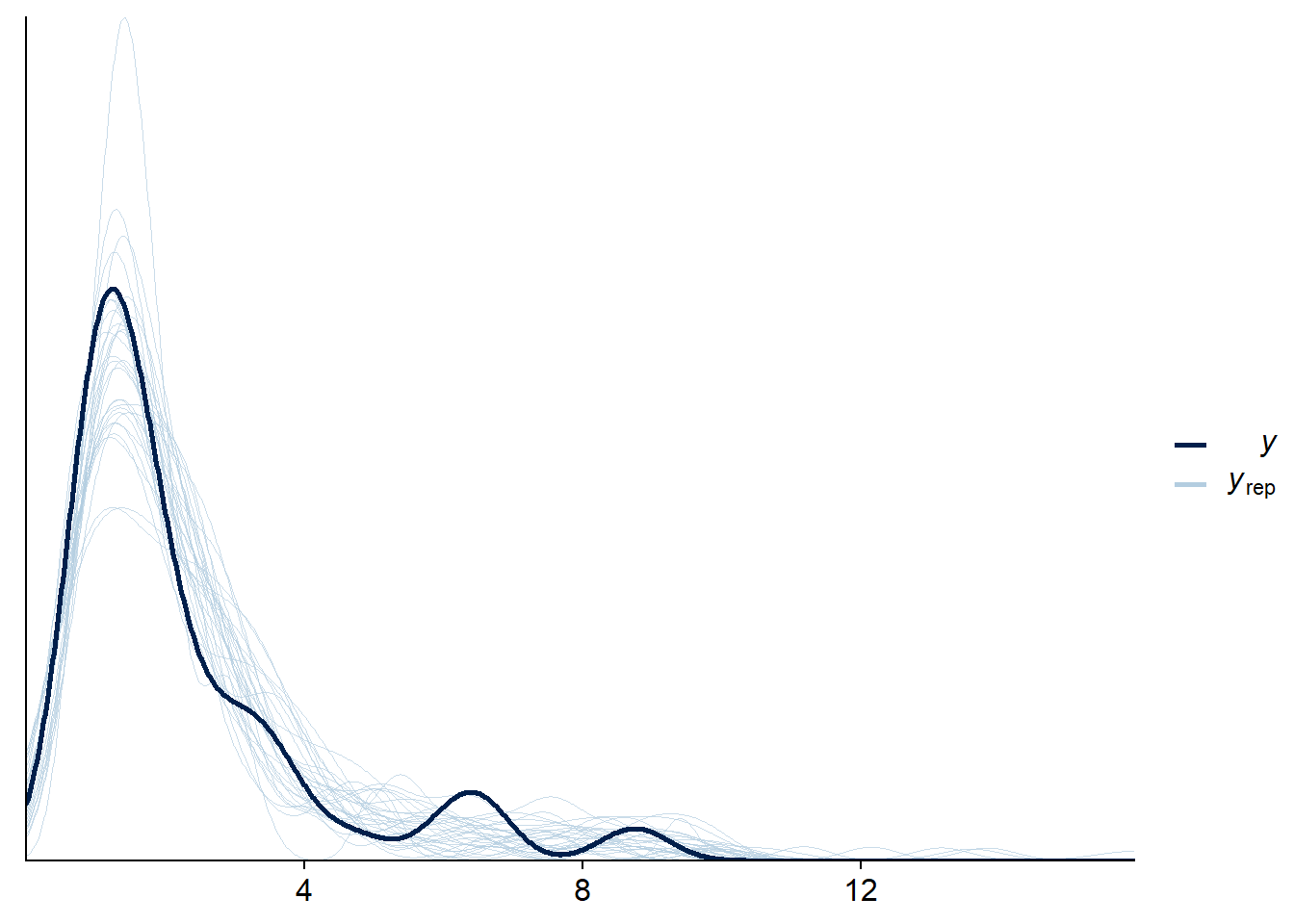

pp_check(fit_mix_multivar, resp = "rt2", ndraws = 30, cores = 1)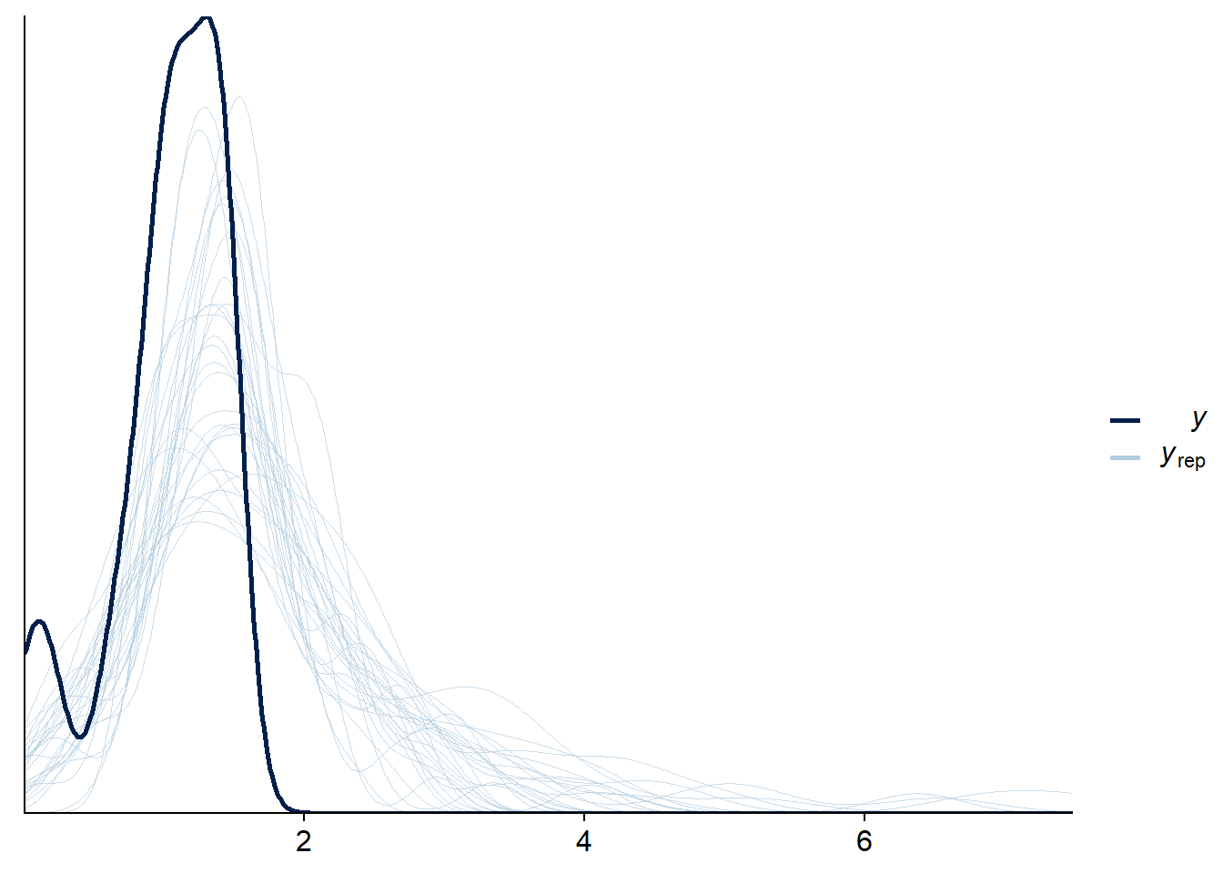

But here we’ll also have to face possibly the biggest problem with brms: that it becomes very easy to specify a model that is too complex to be well informed by the data we have or to even build a completely broken model that no amount of data will save. The data and a few settings for the “crazy” models shown above have actually had to be tweaked for them to work well for this post. So enjoy with moderation :-).

Again, if you want the complete code, packaged in a single file you can just load into your project, go to https://github.com/martinmodrak/blog/blob/master/content/post/RTmixture.R

If you encounter problems running the models that you can’t resolve yourself, be sure to ask questions on Stan Discourse and tag me (@martinmodrak) in the question!

Original computing environment

sessionInfo()

## R version 4.1.0 (2021-05-18)
## Platform: x86_64-w64-mingw32/x64 (64-bit)
## Running under: Windows 10 x64 (build 18363)
## 
## Matrix products: default
## 
## locale:
## [1] LC_COLLATE=English_United States.1252 
## [2] LC_CTYPE=English_United States.1252   
## [3] LC_MONETARY=English_United States.1252
## [4] LC_NUMERIC=C                          
## [5] LC_TIME=English_United States.1252    
## 
## attached base packages:
## [1] stats     graphics  grDevices utils     datasets  methods   base     
## 
## other attached packages:
##  [1] bayesplot_1.8.1     patchwork_1.1.1     knitr_1.33         
##  [4] forcats_0.5.1       stringr_1.4.0       dplyr_1.0.7        
##  [7] purrr_0.3.4         readr_2.0.1         tidyr_1.1.3        
## [10] tibble_3.1.3        ggplot2_3.3.5       tidyverse_1.3.1    
## [13] brms_2.16.2         Rcpp_1.0.7          cmdstanr_0.4.0.9000
## 
## loaded via a namespace (and not attached):
##   [1] readxl_1.3.1         backports_1.2.1      plyr_1.8.6          
##   [4] igraph_1.2.6         splines_4.1.0        crosstalk_1.1.1     
##   [7] rstantools_2.1.1     inline_0.3.19        digest_0.6.27       
##  [10] htmltools_0.5.1.1    rsconnect_0.8.24     fansi_0.5.0         
##  [13] magrittr_2.0.1       checkmate_2.0.0      tzdb_0.1.2          
##  [16] modelr_0.1.8         RcppParallel_5.1.4   matrixStats_0.61.0  
##  [19] xts_0.12.1           prettyunits_1.1.1    colorspace_2.0-2    
##  [22] rvest_1.0.1          haven_2.4.3          xfun_0.25           
##  [25] callr_3.7.0          crayon_1.4.1         jsonlite_1.7.2      
##  [28] lme4_1.1-27.1        zoo_1.8-9            glue_1.4.2          
##  [31] gtable_0.3.0         V8_3.4.2             distributional_0.2.2
##  [34] pkgbuild_1.2.0       rstan_2.26.3         abind_1.4-5         
##  [37] scales_1.1.1         mvtnorm_1.1-2        DBI_1.1.1           
##  [40] miniUI_0.1.1.1       xtable_1.8-4         stats4_4.1.0        
##  [43] StanHeaders_2.26.3   DT_0.18              htmlwidgets_1.5.3   
##  [46] httr_1.4.2           threejs_0.3.3        posterior_1.0.1     
##  [49] ellipsis_0.3.2       pkgconfig_2.0.3      loo_2.4.1           
##  [52] farver_2.1.0         sass_0.4.0           dbplyr_2.1.1        
##  [55] utf8_1.2.2           labeling_0.4.2       tidyselect_1.1.1    
##  [58] rlang_0.4.11         reshape2_1.4.4       later_1.2.0         
##  [61] munsell_0.5.0        cellranger_1.1.0     tools_4.1.0         
##  [64] cli_3.0.1            generics_0.1.0       broom_0.7.9         
##  [67] ggridges_0.5.3       evaluate_0.14        fastmap_1.1.0       
##  [70] yaml_2.2.1           processx_3.5.2       fs_1.5.0            
##  [73] nlme_3.1-152         mime_0.11            projpred_2.0.2      
##  [76] xml2_1.3.2           compiler_4.1.0       shinythemes_1.2.0   
##  [79] rstudioapi_0.13      curl_4.3.2           gamm4_0.2-6         
##  [82] reprex_2.0.1         bslib_0.2.5.1        stringi_1.7.3       
##  [85] highr_0.9            ps_1.6.0             blogdown_1.5        
##  [88] Brobdingnag_1.2-6    lattice_0.20-44      Matrix_1.3-3        
##  [91] nloptr_1.2.2.2       markdown_1.1         shinyjs_2.0.0       
##  [94] tensorA_0.36.2       vctrs_0.3.8          pillar_1.6.2        
##  [97] lifecycle_1.0.0      jquerylib_0.1.4      bridgesampling_1.1-2
## [100] cowplot_1.1.1        httpuv_1.6.1         R6_2.5.0            
## [103] bookdown_0.22        promises_1.2.0.1     gridExtra_2.3       
## [106] codetools_0.2-18     boot_1.3-28          colourpicker_1.1.0  
## [109] MASS_7.3-54          gtools_3.9.2         assertthat_0.2.1    
## [112] withr_2.4.2          shinystan_2.5.0      mgcv_1.8-35         
## [115] parallel_4.1.0       hms_1.1.0            grid_4.1.0          
## [118] coda_0.19-4          minqa_1.2.4          rmarkdown_2.10      
## [121] shiny_1.6.0          lubridate_1.7.10     base64enc_0.1-3     
## [124] dygraphs_1.1.1.6