library(cmdstanr)
library(brms)
library(tidyverse)
library(knitr)
ggplot2::theme_set(cowplot::theme_cowplot())
options(mc.cores = parallel::detectCores(), brms.backend = "cmdstanr")

document_output <- isTRUE(getOption('knitr.in.progress'))

if(document_output) {
  table_format <- knitr::kable
} else {
  table_format <- identity
}

Our contestants

We will keep stuff very simple. Our first contestant, the humble null model a.k.a. \(\mathcal{M}_1\) will be that the \(K\) data points are independent draws from a standard normal distribution, i.e.:

\[ \mathcal{M}_1 : \mathbf{y} = \{y_1, ... , y_K\} \\ y_i \sim N(0,1) \] In code, simulating from such a model this would look like:

N <- 10 # Size of dataset
y <- rnorm(N, mean = 0, sd = 1)

The null model has faced a lot of rejection in their whole life, but has kept its spirit up despite all the adversity. But will it be enough?

The challenger will be the daring intercept model a.k.a. the destroyer of souls a.k.a. \(\mathcal{M}_2\) that posits that there is an unknown, almost surely non-zero mean of the normal distribution, i.e.:

\[ \mathcal{M}_2: \mathbf{y} = \{y_1, ... , y_K\} \\ y_i \sim N(\alpha, 1) \\ \alpha \sim N(0,2) \]

The corresponding R code would be:

N <- 10 # Size of dataset
alpha <- rnorm(1, 0, 2)
y <- rnorm(N, mean = alpha, sd = 1)

This comparison is basically the Bayesian alternative of a single sample t-test with fixed variance - so very simple indeed.

Finally let’s prepare some data for our contestants to chew on:

y <- c(0.5,0.7, -0.4, 0.1)

Method 1: brms::hypothesis

We will start by where most users probably start: invoking a statistical package to compute the Bayes factor. Here we will use the hypothesis function from brms which uses the Savage-Dickey method under the hood.

For this, we note that the null model is just a special case of the intercept model, destroyer of suns. So let us fit this model (\(\mathcal{M}_2\)) in brms. We will be using a lot of samples to reduce estimator error as Bayes factors can be quite sensitive.

cache_dir <- "_bf_cache"
if(!dir.exists(cache_dir)) {
  dir.create(cache_dir)
}

fit_brms <- brm(y ~ 0 + Intercept,  # `0 + Intercept` avoids centering
                prior = 
                  c(prior(normal(0,2), class = b), # Our prior on intercept
                    prior(constant(1), class = sigma)), # Fix sigma to a constant
                data = data.frame(y = y),
                iter = 10000,
                sample_prior = "yes",  # Needed to compute BF
                refresh = 0, silent = TRUE,
                file = paste0(cache_dir, "/fit"), # Cache the results
                file_refit = "on_change")

Hypothesis then gives us two numbers, the Bayes factor of null over intercept (\(BF_{12}\)), a.k.a. evidence ratio and the posterior probability that null model generated the data \(P(\mathcal{M}_1 | \mathbf{y})\):

hyp_res <- hypothesis(fit_brms, "Intercept = 0")
bf_brms <- hyp_res$hypothesis$Evid.Ratio
prob_null_brms <- hyp_res$hypothesis$Post.Prob
res_brms <- data.frame(method = "brms", bf = bf_brms, prob_null = prob_null_brms)
res_brms %>% table_format

method	bf	prob_null
brms	3.898489	0.7958554

Those two qunatities happen to share a pretty straightforward relationship, given the prior probabilities of the individual models \(P(\mathcal{M}_1)\), \(P(\mathcal{M}_2)\) i.e.:

\[ P(\mathcal{M}_1 | \mathbf{y}) = \frac{BF_{12}P(\mathcal{M}_1)}{BF_{12}P(\mathcal{M}_1) + BF_{22}P(\mathcal{M}_2)} = \\ = \frac{BF_{12}P(\mathcal{M}_1)}{BF_{12}P(\mathcal{M}_1) + P(\mathcal{M}_2)} \] Where \(BF_{22} = 1\) is the Bayes factor of the intercept model, cruel queen of the damned, against itself. If the prior is uniform, i.e. \(P(\mathcal{M}_1) = P(\mathcal{M}_2)\) - as is assumed by brms - the formula further simplifies to:

\[ P(\mathcal{M}_1 | \mathbf{y}) = \frac{BF_{12}}{BF_{12} + 1} \]

The Bayes factor might look a bit like a magic number, so let us demystify it with two more transparent approaches that give us the same Bayes factor.

Method 2: Prior predictive density

One way to define Bayes factor is as the ratio of evidence i.e.:

\[ BF_{12} = \frac{P(\mathbf{y} | \mathcal{M}_1)}{P(\mathbf{y} | \mathcal{M}_2)} \]

Where “evidence” is exactly the prior density of the data after integrating out all the parameters. Since we have chosen very simple models, there is an analytic formula for evidence for both models.

As is usually done for numerical stability, we will primarily operate on the log scale. Computing the evidence for the null model is straightforward - there are no parameters to integrate out, so we can directly compute:

prior_log_evidence_null <- sum(dnorm(y, mean = 0, sd = 1, log = TRUE))
prior_log_evidence_null

## [1] -4.130754

The evidence for the intercept model, prophet of the apocalypse, is slightly more involved. The main idea is that we can see the data as sum of two multivariate normals, one with perfect correlation (corresponding to \(K\) identical copies of \(\alpha\)) and one with no correlation (corresponding to noise):

\[ \mathcal{M}_2: \mathbf{y} = \mathbf{a} + \mathbf{e} \\ \mathbf{a} \sim MVN(0, \mathbf{\Sigma_a}), \forall_{i,j \in \{1, .., K\}} \Sigma_{a;i,j} = Var(\alpha) = 4 \\ \mathbf{e} \sim MVN(0, \mathbf{\Sigma_e}), \mathbf{\Sigma_{e}} = I \\ \]

where \(\mathbf{\Sigma_a}\) is a matrix with all elements set to \(Var(\alpha) = 4\) and \(\mathbf{\Sigma_e}\) is the identity matrix (1 on diagonal, 0 elsewhere). From the properties of multivariate normal we know that a sum of multivariate normals is obtained by simply adding both means and covariance matrices together, i.e.:

\[ \mathcal{M}_2: \mathbf{y} \sim MVN(0, \mathbf{\Sigma}) \\ \forall_{i \in \{1, .., K\}}\mathbf{\Sigma}_{i,i} = 5 \\ \forall_{i \neq j \in \{1, .., K\}} \mathbf{\Sigma}_{i,j} = 4 \]

where \(\mathbf{\Sigma} = \mathbf{\Sigma_a} + \mathbf{\Sigma_e}\). With that we can compute the evidence for the intercept model, the harbinger of sorrow, \(P(\mathbf{y} | \mathcal{M}_2)\) as the corresponding multivariate normal density:

prior_Sigma <- diag(length(y)) + matrix(4, nrow = length(y), ncol = length(y))
prior_log_evidence_intercept <- 
  mvtnorm::dmvnorm(y, mean = rep(0, length(y)), sigma = prior_Sigma, log = TRUE)

prior_log_evidence_intercept

## [1] -5.452067

The Bayes factor is then simply the ratio of the evidence and we can use the BF to compute the posterior probability of the null model, assuming once again uniform prior.

bf_prior <- exp(prior_log_evidence_null - prior_log_evidence_intercept)
prob_null_prior <- bf_prior / (bf_prior + 1)
res_prior <- data.frame(method = "prior", bf = bf_prior, prob_null = prob_null_prior)
rbind(res_prior, res_brms) %>% table_format

method	bf	prob_null
prior	3.748338	0.7894000
brms	3.898489	0.7958554

We see the results happen to match pretty closely with the value obtained via brms. The difference can be attributed to sampling error in the brms computation.

Method 3: Supermodel

A third perspective is provided by imagining a “supermodel” combining our two contestants, i.e.:

\[ \mathcal{M}_{super}: \mathbf{y} = \{y_1, ... , y_K\} \\ z \in \{1,2\}; P(z = 1) = P(z = 2) = \frac{1}{2}\\ y_i \sim N(\mu, 1) \\ \mu = \begin{cases} 0 & \mathrm{if} \quad z = 1 \\ \alpha & \mathrm{if} \quad z = 2 \end{cases} \\ \alpha \sim N(0,2) \] So we have introduced a new random variable \(z\) that works as an index over the two models and gave it a discrete uniform prior.

If we fit this model to the data, then \(P(\mathcal{M}_1 | \mathbf{y}) = P(z = 1 | \mathbf{y})\), so we can use the fitted distribution of \(z\) to get the posterior probability of the models which (as shown above) we can transform into a Bayes factor.

Before showing how to do this in Stan, we can use JAGS to implement this model very directly, if not very efficiently:

suppressPackageStartupMessages(library(rjags))

## Warning: package 'rjags' was built under R version 4.3.3

data_list <- list(
    y = y)

# The model specification, note that JAGS uses precision
# to parametrize normal distribution
# Additionally we have z_0 = z - 1
jags_model_string <- "model {
  z_0 ~ dbern(0.5) 
  alpha ~ dnorm(0, 0.25)
  for(i in 1:length(y) ) {
    mu[i] = ifelse(z_0 == 0, 0, alpha)
    y[i] ~ dnorm(mu[i], 1)
  } 
}"

params_to_monitor <- c("z_0", "alpha")

# Running the model
model <- jags.model( textConnection(jags_model_string), data_list, 
                     n.chains = 4, n.adapt= 1000)

## Compiling model graph
##    Resolving undeclared variables
##    Allocating nodes
## Graph information:
##    Observed stochastic nodes: 4
##    Unobserved stochastic nodes: 2
##    Total graph size: 12
## 
## Initializing model

update(model, 1000); # Burning 1000 samples to the MCMC gods...
mcmc_samples <- coda.samples(model, params_to_monitor, n.iter=10000, thin = 10)

# Extract values and check diagnostics
alpha_array <- cbind(mcmc_samples[[1]][, "alpha"], mcmc_samples[[2]][, "alpha"],
                     mcmc_samples[[3]][, "alpha"], mcmc_samples[[4]][, "alpha"])
posterior::rhat(alpha_array)

## [1] 1.00007

posterior::ess_bulk(alpha_array)

## [1] 3802.998

z_array <- cbind(mcmc_samples[[1]][, "z_0"], mcmc_samples[[2]][, "z_0"],
                 mcmc_samples[[3]][, "z_0"], mcmc_samples[[4]][, "z_0"])
posterior::rhat(z_array)

## [1] 1.000246

posterior::ess_bulk(z_array)

## [1] 3962.832

Posterior probability of the data being from the null model (\(P(\mathcal{M}_1 | \mathbf{y})\)), is then simply the \(P(z = 1 | \mathbf{y}) = P(z_0 = 0 | \mathbf{y})\) which can be directly extracted from the samples.

prob_null_jags <- mean(z_array == 0)
bf_jags <- prob_null_jags / (1 - prob_null_jags)
res_jags <- data.frame(method = "super_jags", bf = bf_jags, 
                       prob_null = prob_null_jags)
rbind(res_jags, res_prior, res_brms) %>% table_format()

method	bf	prob_null
super_jags	3.711425	0.7877500
prior	3.748338	0.7894000
brms	3.898489	0.7958554

We once again see a good agreement.

But we obviously want to do this in Stan. But Stan doesn’t handle discrete parameters you say? This can be overcome!

Warning: I had a lot of trouble thinking clearly about the rest of this section, so it is possible, there are mistakes or stuff is confusing. Please let me know, if you find the reasoning problematic/unclear/unconvincing.

The important point is called marginalization and there is a neat intro to it in the preprint for the rater package. More discussion and examples are in the Stan User’s guide. The point is that we can express the unnormalized density \(p(\alpha, \mathbf{y})\) as:

\[ \mathcal{M}_{super-marginalized}: \\ p(\alpha, \mathbf{y}) = p(\alpha)p(\mathbf{y}| \alpha) \\ p(\mathbf{y}| \alpha) = p(\mathbf{y} | \alpha, z = 1)p(z = 1) + p(\mathbf{y} | \alpha, z = 1)p(z = 0) \] Now we have a density for \(y\) that is a combination of two normal densities and does not have \(z\) as a free parameter and can thus be written in Stan as:

cat(readLines("2021-bayes-factors.stan"), sep = "\n")

data {
  int K;
  vector[K] y;
}

parameters {
  real alpha;
}

transformed parameters {
  real log_lik_null = normal_lpdf(y | 0, 1);
  real log_lik_intercept = normal_lpdf(y | alpha, 1);
}

model {
    target += log_mix(0.5, log_lik_null, log_lik_intercept);
    target += normal_lpdf(alpha | 0, 2);
}

super_model <- cmdstan_model("2021-bayes-factors.stan")

But how do we get back to the value we are actually interested in, that is \(P(z = 1 | \mathbf{y})\) when there no longer is any \(z\)?

We can use the Bayes rule and since \(z\) and \(\alpha\) are a-prior independent, we can assume \(P(z = 1 | \alpha) = P(z = 1) = \frac{1}{2}\). This gives:

\[ P(z = 1 | \mathbf{y}, \alpha) =\\ = \frac{P(z = 1 | \alpha) \times p(\mathbf{y} | z = 1, \alpha)}{P(z = 1 | \alpha) \times p(\mathbf{y} | z = 1, \alpha) + P(z = 2 | \alpha) \times p(\mathbf{y} | z = 2, \alpha)} = \\ =\frac{\frac{1}{2} p(\mathbf{y} | z = 1)}{\frac{1}{2} p(\mathbf{y} | z = 1) + \frac{1}{2} p(\mathbf{y} | z = 2, \alpha)} \]

So to get the desired \(P(z = 1 | \mathbf{y})\) I need to integrate out \(\alpha\), which I can approximate via posterior samples:

\[ P(z = 1 | \mathbf{y}) = \int P(z = 1 | \mathbf{y}, \alpha) \mathrm{d} \alpha \simeq \frac{1}{M} \sum_m P(z = 1 | \mathbf{y}, \alpha = \alpha_m) \]

So let us fit the model:

fit_super <- super_model$sample(
  data = list(K = length(y), y = y), refresh = 0, iter_sampling = 10000)

## Running MCMC with 4 chains, at most 12 in parallel...
## 
## Chain 1 finished in 0.3 seconds.
## Chain 2 finished in 0.3 seconds.
## Chain 3 finished in 0.2 seconds.
## Chain 4 finished in 0.3 seconds.
## 
## All 4 chains finished successfully.
## Mean chain execution time: 0.3 seconds.
## Total execution time: 0.5 seconds.

fit_super$summary() %>% table_format()

variable	mean	median	sd	mad	q5	q95	rhat	ess_bulk	ess_tail
lp__	-6.5619847	-6.4162500	0.847365	0.7940064	-8.159686	-5.703508	1.000154	11044.62	12052.58
alpha	0.0490804	0.0948292	1.793511	1.4701640	-3.034274	3.098635	1.000182	11120.88	11475.93
log_lik_null	-4.1307500	-4.1307500	0.000000	0.0000000	-4.130750	-4.130750	NA	NA	NA
log_lik_intercept	-10.5246013	-6.0134100	10.546830	2.8471109	-32.070390	-4.041240	1.000103	10990.77	12359.95

No warnings, rhat and ess look good. Now, let’s extract the partial likelihoods and combine them into the BMA weight:

super_samples <-posterior::as_draws_matrix(fit_super$draws())

rel_p_null <- exp(super_samples[,"log_lik_null"])
rel_p_intercept <- exp(super_samples[,"log_lik_intercept"])
prob_null_stan <- mean(rel_p_null / (rel_p_null + rel_p_intercept))

bf_stan <-  prob_null_stan / (1 - prob_null_stan) 

res_stan <- data.frame(
  method = "super_stan", bf = bf_stan, prob_null = prob_null_stan)
rbind(res_stan, res_jags, res_prior, res_brms) %>% table_format()

method	bf	prob_null
super_stan	3.753493	0.7896284
super_jags	3.711425	0.7877500
prior	3.748338	0.7894000
brms	3.898489	0.7958554

By marginalizing, we are not only having a model with fewer parameters (and hence simpler to sample), we are also able to better resolve tails: if I have 1000 samples of \(z\), I cannot reliably estimate if \(P(z = 1) < 10^{-3}\) - I will just see that none (or almost none) samples are \(1\). After marginalizing, each sample gives me directly a sample of \(P(z = 1)\), so I can get reasonable precision even if \(P(z = 1)\) is very close to \(0\) or \(1\).

Viewing Bayes factors as derived from posterior probabilities of an index over candidate models (\(z\) in our case), puts a different angle on the distinction between \(\mathcal{M}\)-closed scenarios (the true model is among the models we compare) and \(\mathcal{M}\)-open / \(\mathcal{M}\)-complete where this is not the case.

If we treat the model selection as fitting the super model with the candidates as submodels, being in an \(\mathcal{M}\)-open scenario simply means that the super model is misspecified. Unfortunately, as discussed above, Bayes factors can be very sensitive to both prior and likelihood specification, where other approaches, e.g. approximate leave-one-out cross validation with loo is usually less sensitive to priors and less often overconfident in face of misspecifaction (see e.g. Using Stacking to Average Bayesian Predictive Distributions by Yao et al. for more discussion).

But we have many good ways to detect model misspecification, including prior and posterior predictive checks and other steps outlined in the Bayesian workflow preprint. So it would be interesting to test whether there is something to be gained by running prior and posterior predictive checks (or other diagnostics), not only for the component models, but for the “supermodel” implied by the selection scheme. But I’ll that to people who actually want to use Bayes factors :-D.

I’ll further note that I tried to implemented a supermodel with two realistic models and it appears that such supermodels can be challenging to fit (my impression is that the problem is primarily in initialization, but I didn’t investigate thoroughly).

Broader comparison

Above, we computed the Bayes factors only for one dataset, so you might not be convinced that the agreement holds for any dataset. So here we’ll encapsulate the code in a few functions and evaluate a bit larger sample.

bf_brms <- function(y) {
  fit_new <- update(fit_brms, newdata = data.frame(y = y), refresh = 0)
  hyp_res <- hypothesis(fit_new, "Intercept = 0")
  bf_brms <- hyp_res$hypothesis$Evid.Ratio
  prob_null_brms <- hyp_res$hypothesis$Post.Prob
  data.frame(method = "brms", bf = bf_brms, prob_null = prob_null_brms)
}

bf_prior <- function(y) {
  prior_log_evidence_null <- sum(dnorm(y, mean = 0, sd = 1, log = TRUE))
  prior_Sigma <- diag(length(y)) + matrix(4, nrow = length(y), ncol = length(y))
  prior_log_evidence_intercept <- 
      mvtnorm::dmvnorm(y, mean = rep(0, length(y)), sigma = prior_Sigma, log = TRUE)
  bf_prior <- exp(prior_log_evidence_null - prior_log_evidence_intercept)
  prob_null_prior <- bf_prior / (bf_prior + 1)

  data.frame(method = "prior", bf = bf_prior, prob_null = prob_null_prior)
}

bf_super_stan <- function(y) {
  fit_super <- super_model$sample(data = list(K = length(y), y = y), refresh = 0, 
                                iter_sampling =  10000)
  
  super_samples <-posterior::as_draws_matrix(fit_super$draws())
  
  rel_p_null <- exp(super_samples[,"log_lik_null"])
  rel_p_intercept <- exp(super_samples[,"log_lik_intercept"])
  p_null <- mean(rel_p_null / (rel_p_null + rel_p_intercept))
  
  
  bf <- p_null / (1 - p_null) # The Bayes factor
  data.frame(method = "super_Stan", bf = bf, prob_null = p_null)
}

bf_super_jags <- function(y) {
  data_list <- list(
    y = y)
  params_to_monitor <- c("z_0", "alpha")

  # Running the model
  model <- jags.model( textConnection(jags_model_string), data_list, 
                       n.chains = 4, n.adapt= 1000)
  update(model, 1000); # Burning 1000 samples to the MCMC gods...
  mcmc_samples <- coda.samples(model, params_to_monitor, n.iter=10000, thin = 10)
  
  z_array <- cbind(mcmc_samples[[1]][, "z_0"], mcmc_samples[[2]][, "z_0"],
                   mcmc_samples[[3]][, "z_0"], mcmc_samples[[4]][, "z_0"])
  
  prob_null_jags <- mean(z_array == 0)
  prob_null_jags
  bf_jags <- prob_null_jags / (1 - prob_null_jags)
  bf_jags
  data.frame(method = "super_jags", bf = bf_jags, prob_null = prob_null_jags)
}

comparisons_file <- paste0(cache_dir, "/comparison.rds")
if(!file.exists(comparisons_file)) {
  set.seed(3384528)
  res_list <- list()
  for(i in 1:50) {
    use_null <- (i %% 2) == 0
    N <- 2 +  rnbinom(1, mu = 10, size = 1)
    if(use_null) {
      mu <- 0
    } else {
      mu <- rnorm(1, 0, 2)
    }
    y <- rnorm(10, mu, sd = 1)
    res_list[[i]] <- rbind(bf_prior(y), 
                           bf_brms(y), 
                           bf_super_jags(y), 
                           bf_super_stan(y)) 
    res_list[[i]]$id = i
    res_list[[i]]$null_true = use_null
    res_list[[i]]$N = N
  }
  res <- do.call(rbind, res_list)
  saveRDS(res, comparisons_file)
} else {
  res <- readRDS(comparisons_file)
}

We note that some Bayes factors - exclusively those computed by the unmarginalized JAGS model are 0. This is unsurprising, as the 10000-iteration JAGS model loses ability to capture very low null probabilities and hence low Bayes factors - looking at the analytically computed Bayes factors of those problematic results they are invariably very low.

# Contrast the BFs with the "prior" (analytically computed) 
comparisons_to_plot <- res %>% group_by(id) %>%
  mutate(bf_prior = bf[method == "prior"], 
         prob_null_prior = bf[method == "prior"]) %>%
  ungroup() %>%
  filter(method != "prior")

zero_bf <- comparisons_to_plot %>% filter(bf == 0)
if(!identical(unique(zero_bf$method), "super_jags")){
  stop("Bad assumption")
}
nrow(zero_bf)

## [1] 11

zero_bf$bf_prior

##  [1] 1.242613e-37 3.423453e-23 3.619076e-09 1.497207e-21 4.917385e-10
##  [6] 2.431973e-14 2.176901e-20 2.514081e-53 1.366711e-13 8.921497e-07
## [11] 1.321580e-05

We’ll exclude those invalid Bayes factors from further consideration.

comparisons_to_plot <- comparisons_to_plot %>% filter(bf > 0)

We can now plot the results of the various Monte carlo methods against the analytical results:

base_comparisons_plot <- function(comparisons, x, y, trans, breaks = waiver()) {
comparisons %>% 
  sample_frac() %>% #random reorder
  ggplot(aes(x = {{x}}, y = {{y}}, color = method, shape = method)) +
  geom_abline(slope = 1, intercept = 0, color = "black") +
  geom_point(size = 3, alpha = 0.8) +
  guides(color = guide_legend(override.aes = list(alpha = 1))) +
  scale_x_continuous(trans = trans, breaks = breaks) +
  scale_y_continuous(trans = trans, breaks = breaks)
  
}

base_comparisons_plot(comparisons_to_plot, bf_prior, bf, trans = "log",
                      breaks = c(1e-45, 1e-30,1e-15, 1))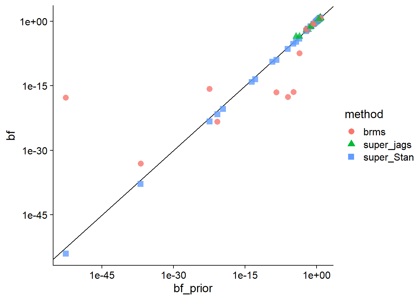

We immediately see that only the marginalized Stan model keeps high agreement for the very low Bayes factors (yay marginalization!).

We can also zoom in on the upper-right area, where we see pretty good agreement between all methods.

base_comparisons_plot(comparisons_to_plot %>% filter(bf_prior > 1e-3), 
                      bf_prior, bf, trans = "log",
                      breaks = c(1e-3, 1e-2,1e-1, 1, 10))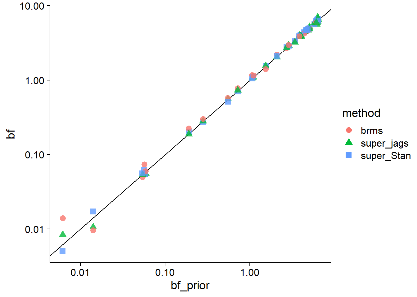

Calibration

Following the method outline by Schad et al. we also check the calibration of our Bayes factors. Since the model has analytical solution, our simulations are going to be much cheaper than in actual practice and we can do a lot of them.

  N_calibration <- 20 # How many values in a dataset
  set.seed(5487654)
  res_cal_list <- list()
  for(i in 1:5000) {
    use_null <- (i %% 2) == 0
    if(use_null) {
      mu <- 0
    } else {
      mu <- rnorm(1, 0, 2)
    }
    y <- rnorm(N_calibration, mu, sd = 1)
    res_cal_list[[i]] <- bf_prior(y)
    res_cal_list[[i]]$null_true = use_null
  }
  calibration <- do.call(rbind, res_cal_list)

As a quick heuristic, reflecting some common usage, we will interpret BF > 3 as weak evidence and BF > 10 as strong evidence. If we do this, this is how our results look like based on whether the null is actually true:

calibration %>% group_by(null_true) %>%
  summarise(strong_null = mean(bf >= 10),
            weak_null = mean(bf >= 3 & bf < 10),
            no_evidence = mean(bf < 3 & bf > 1/3), 
            weak_intercept = mean(bf <= 1/3 & bf > 0.01),
            strong_intercept = mean(bf <= 0.01), .groups = "drop") %>%
  table_format()

null_true	strong_null	weak_null	no_evidence	weak_intercept	strong_intercept
FALSE	0	0.1364	0.0852	0.0924	0.686
TRUE	0	0.8572	0.1328	0.0100	0.000

We see that in the case of observing 20 values, this simple heuristic makes a potentially non-intuitive trade-off where low rates of wrongly claiming support for the intercept model, the maternal uncle of despair, are balanced by low rates of correctly finding strong support for the null model and by somewhat large rate of finding weak evidence in favor of the null model, even when this model was not used to simulate data.

This is just to illustrate the point made by Schad et al. that explicit calibration and decision analysis should be done in the context of a given experimental design and utility/cost of actual decisions. But wan can be safe in the knowledge that the poor null model is unlikely to suffer unjust rejections in this case.

Conclusions

Bayes factors are not very intuitive, but I hope that understanding that the same number can be understood as either being a ratio of prior predictive densities or from a larger model taking the candidate models as components could help improve the intuition. In line with the (better, more thoroughly done) results of Schad et al. we also observe that computation of Bayes factors cannot be taken for granted and that simple heuristics to interpret Bayes factors may have non-obvious implications.

Now go read Workflow Techniques for the Robust Use of Bayes Factors!

UPDATE: I have a followup post discussing the connection between Bayes factors and cross-validation on the same examples.