Setting up

Let’s set up and get our hands dirty.

library(cmdstanr)
library(brms)
library(tidyverse)
library(knitr)
library(bayesplot)

ggplot2::theme_set(cowplot::theme_cowplot())
options(mc.cores = parallel::detectCores(), brms.backend = "cmdstanr")

cache_dir <- "_brms_ranef_cache"
if(!dir.exists(cache_dir)) {
  dir.create(cache_dir)
}

Simulate data

Note that the way we have setup the model implies that patients are nested within treatments (i.e. that each patient only ever gets one treatment). Since each random effect can only have one prior distribution, this is the easiest way to make sense of the model.

First, we setup the treatment-level predictors in a treatment-level data frame and use those to predict the sds (\(\tau\) above).

set.seed(354855)
N <- 500
N_pts <- floor(N / 5)
N_trts <- 10
trt_intercept <- 0
trt_x_b <- 1
trt_data <- data.frame(trt_x = rnorm(N_trts))
# Corresponds to tau in the mathematical model
trt_sd <- exp(trt_intercept + trt_x_b * trt_data$trt_x)

Now, we setup the patient-level random effects, with varying sds (corresponding to \(\gamma\) above).

patient_treatment <- sample(1:N_trts, size = N_pts, replace = TRUE)
ranef <- rnorm(N_pts, mean = 0, sd = trt_sd[patient_treatment])

Finally, we setup the main data frame with multiple observations of each patient.

intercept <- 1
x_b <- 0.5
obs_sigma <- 1
base_data <- data.frame(x = rnorm(N), 
                        patient_id = rep(1:N_pts, length.out = N))

base_data$trt_id <- patient_treatment[base_data$patient_id]

base_data_predictor <- intercept + x_b * base_data$x + ranef[base_data$patient_id]
base_data$y <- rnorm(N, mean = base_data_predictor , sd = obs_sigma)

Using non-linear formulas

As noted by Ven Popov, we can use non-linear brms formulas for this task. First, we extend the patient-level data with treatment level-data.

trt_with_id <- trt_data %>% mutate(trt_id = 1:n())
data_joined <- base_data %>% inner_join(trt_with_id, by = "trt_id")

Now, we create a patient-level random intercept, but fix its standard deviation to \(1\). We then create a linear predictor for the variance and multiply the “standardized” random intercept with exp-transformed value of the predictor, giving us a random intercept with the correct standard deviation.

This is how the brms code looks like:

# Fix the sd to 1
prior_nl <- prior(constant(1), class='sd', nlpar='patientintercept')


fit_nl <- brm(
     # combine the main predictor with the random effect in a non-linear formula    
  bf(y ~ muy + patientintercept * exp(logmysigma), 
         # main linear predictor for y (additional predictors go here)
         muy ~ x,                                  
         # specify the random intercept
         patientintercept ~ 0 + (1|patient_id),    
         # linear predictor for log random effect sd 
         # (additional predictors for sd go here)
         logmysigma ~ trt_x,                       
         nl = T),
  prior = prior_nl,
  data = data_joined,
  file = file.path(cache_dir, "fit_nl.rds"),
  file_refit = "on_change"
)

We get a decent recovery of the parameters — recall that we simulated data with muy_Intercept = 1, logmysigma_Intercept = 0, muy_x = 0.5, logmysigma_trt_x = 1 and sigma = 1.

summary(fit_nl)

##  Family: gaussian 
##   Links: mu = identity; sigma = identity 
## Formula: y ~ muy + patientintercept * exp(logmysigma) 
##          muy ~ x
##          patientintercept ~ 0 + (1 | patient_id)
##          logmysigma ~ trt_x
##    Data: data_joined (Number of observations: 500) 
##   Draws: 4 chains, each with iter = 2000; warmup = 1000; thin = 1;
##          total post-warmup draws = 4000
## 
## Group-Level Effects: 
## ~patient_id (Number of levels: 100) 
##                                Estimate Est.Error l-95% CI u-95% CI Rhat
## sd(patientintercept_Intercept)     1.00      0.00     1.00     1.00   NA
##                                Bulk_ESS Tail_ESS
## sd(patientintercept_Intercept)       NA       NA
## 
## Population-Level Effects: 
##                      Estimate Est.Error l-95% CI u-95% CI Rhat Bulk_ESS
## muy_Intercept            0.99      0.09     0.80     1.17 1.00     1066
## muy_x                    0.54      0.05     0.45     0.64 1.00     5005
## logmysigma_Intercept     0.17      0.12    -0.07     0.39 1.01      678
## logmysigma_trt_x         0.92      0.10     0.74     1.13 1.01      401
##                      Tail_ESS
## muy_Intercept            1969
## muy_x                    3006
## logmysigma_Intercept     1188
## logmysigma_trt_x          829
## 
## Family Specific Parameters: 
##       Estimate Est.Error l-95% CI u-95% CI Rhat Bulk_ESS Tail_ESS
## sigma     0.96      0.03     0.90     1.03 1.00     3333     2669
## 
## Draws were sampled using sample(hmc). For each parameter, Bulk_ESS
## and Tail_ESS are effective sample size measures, and Rhat is the potential
## scale reduction factor on split chains (at convergence, Rhat = 1).

The hacker’s way

To keep the lessons for future, I am also including a more hacky approach, that in principle lets you do much more, but is a bit of an overkill here. The main downside of my approach is that it forces you to completely override the likelihood and that you have to build the random effect with predicted sigma in hand-written Stan code. This may mean the benefits of brms are now too small and you might be better off building the whole thing directly in Stan.

The first problem to solve is that at its core, brms requires us to use a single data frame as input. But we have a treatment-level data frame and then an observation-level data frame. We get around this by adding dummy values so that both data frames have the same columns, binding the together and then using the subset addition term to use different formulas for each. We will also need a dummy outcome variable for the treatment-level data.

combined_data <- rbind(
  base_data %>% mutate(
    is_trt = FALSE,
    trt_x = 0,
    trt_y = 0
  ),
  trt_data %>% mutate(
    is_trt = TRUE,
    trt_id = 0,
    patient_id = 0,
    y = 0,
    x = 0,
    trt_y = 0
  )
)

The main idea for implementation is that we completely overtake the machinery of brms after the linear predictors are constructed. To do that, we create a custom family that is empty (i.e. adds nothing to the log likelihood) and use it in our formula.

# Build the empty families --- one has just a single parameter and will be used 
# for treatment-level sds. The other has mu and sigma parameter will be used
# for the observation model.
empty_for_trt <- custom_family("empty_for_trt", type = "real")
empty_for_obs <- custom_family("empty_for_obs",  dpars = c("mu", "sigma"), 
                               links = c("identity", "log"), type = "real", lb = c(NA, 0))

empty_func_stanvar <- stanvar(block = "functions", scode = "
  real empty_for_trt_lpdf(real y, real mu) {
    return 0;
  } 
  
  real empty_for_obs_lpdf(real y, real mu, real sigma) {
    return 0;
  }
")

We then take the linear predictions for the sd of the random effects (\(\tau\)) and use it to manually build our random effect values (with non-centered parametrization). We manually add those values to the rest of the linear predictor term and then manually add our desired likelihood.

This will let our final formula to look this way:

f <- mvbrmsformula(
    brmsformula(y | subset(!is_trt)  ~ x, family = empty_for_obs),
    brmsformula(trt_y | subset(is_trt)  ~ trt_x, family = empty_for_trt),
    rescor = FALSE)

In this setup, brms will build a bunch of variables for both formulas that we can access in our Stan code. Their names will depend on the name of the outcome variables — since our main outcome is y, relevant variables will be N_y (number of rows for this outcome), mu_y and sigma_y (distributional parameters for this outcome).

Our dummy outcome is trt_y and the relevant variables will be N_trty and mu_trty, because brms removes underscores. You can always use make_stancode and make_standata to see how brms transforms names and input data.

For all this to happen we also need to pass a bunch of extra data via stanvars.

Let us prepare the extra Stan code.

# Pass the extra data. We'll take advantage of some already existing data
# variables defined by brms, these include:
# N_y - the number of observation-level data 
# N_trty - the number of treatment-level data (and thus the number of treatments)
# we however need to pass the rest of the data for the random effect
data_stanvars <- 
  stanvar(x = N_pts, block = "data", scode = "int<lower=2> N_pts;") +
  stanvar(x = patient_treatment, name = "trt_id", block = "data", 
          scode = "array[N_pts] int<lower=1, upper=N_trty> trt_id;") +
  stanvar(x = base_data$patient_id, name = "patient_id", block = "data", 
          scode = "array[N_y] int<lower=1, upper=N_pts> patient_id;")

# Raw parameters for the random effects
parameter_stanvar <- 
  stanvar(block = "parameters", scode = "
      vector[N_pts] my_ranef_raw;
      ")

# Prior - we are using the non-centered parametrization, so it is just N(0,1)
# and we multiply by the sd later.
# Note that current versions of brms compute log-prior in the transformed
# parameters block, so we do it as well.
prior_stanvar <-
  stanvar(block = "tparameters", 
          scode = "lprior += std_normal_lpdf(to_vector(my_ranef_raw));")

# Here is where we add the random effect to the existing predictor values and 
# reconstruct the likelihood.
# Once again using the values generated by brms for the predictors in mu_trty,
# mu_y, sigma_y.
likelihood_stanvar <- 
  stanvar(block = "likelihood", position = "end", scode = "
      // New scope to let us introduce new parameters
      {
          vector[N_trty] trt_sds = exp(mu_trty);
          vector[N_pts] my_ranef = my_ranef_raw .* trt_sds[trt_id];
          for(n in 1: N_y) {
            // Add the needed ranef 
            real mu_with_ranef = mu_y[n] + my_ranef[patient_id[n]];
            // reimplement the likelihood
            target += normal_lpdf(Y_y[n] | mu_with_ranef, sigma_y);
          }
      }
          ") 
  

predict_ranef_stanvars <- empty_func_stanvar + 
  data_stanvars + 
  parameter_stanvar + 
  prior_stanvar +
  likelihood_stanvar

This is the complete Stan code generated by brms with our additions:

make_stancode(f, data = combined_data,
  stanvars = predict_ranef_stanvars)

## // generated with brms 2.20.4
## functions {
##   real empty_for_trt_lpdf(real y, real mu) {
##     return 0;
##   }
##   
##   real empty_for_obs_lpdf(real y, real mu, real sigma) {
##     return 0;
##   }
## }
## data {
##   int<lower=1> N; // total number of observations
##   int<lower=1> N_y; // number of observations
##   vector[N_y] Y_y; // response variable
##   int<lower=1> K_y; // number of population-level effects
##   matrix[N_y, K_y] X_y; // population-level design matrix
##   int<lower=1> Kc_y; // number of population-level effects after centering
##   int<lower=1> N_trty; // number of observations
##   vector[N_trty] Y_trty; // response variable
##   int<lower=1> K_trty; // number of population-level effects
##   matrix[N_trty, K_trty] X_trty; // population-level design matrix
##   int<lower=1> Kc_trty; // number of population-level effects after centering
##   int prior_only; // should the likelihood be ignored?
##   int<lower=2> N_pts;
##   array[N_pts] int<lower=1, upper=N_trty> trt_id;
##   array[N_y] int<lower=1, upper=N_pts> patient_id;
## }
## transformed data {
##   matrix[N_y, Kc_y] Xc_y; // centered version of X_y without an intercept
##   vector[Kc_y] means_X_y; // column means of X_y before centering
##   matrix[N_trty, Kc_trty] Xc_trty; // centered version of X_trty without an intercept
##   vector[Kc_trty] means_X_trty; // column means of X_trty before centering
##   for (i in 2 : K_y) {
##     means_X_y[i - 1] = mean(X_y[ : , i]);
##     Xc_y[ : , i - 1] = X_y[ : , i] - means_X_y[i - 1];
##   }
##   for (i in 2 : K_trty) {
##     means_X_trty[i - 1] = mean(X_trty[ : , i]);
##     Xc_trty[ : , i - 1] = X_trty[ : , i] - means_X_trty[i - 1];
##   }
## }
## parameters {
##   vector[Kc_y] b_y; // regression coefficients
##   real Intercept_y; // temporary intercept for centered predictors
##   real<lower=0> sigma_y; // dispersion parameter
##   vector[Kc_trty] b_trty; // regression coefficients
##   real Intercept_trty; // temporary intercept for centered predictors
##   
##   vector[N_pts] my_ranef_raw;
## }
## transformed parameters {
##   real lprior = 0; // prior contributions to the log posterior
##   lprior += std_normal_lpdf(to_vector(my_ranef_raw));
##   lprior += student_t_lpdf(Intercept_y | 3, 0.9, 2.5);
##   lprior += student_t_lpdf(sigma_y | 3, 0, 2.5)
##             - 1 * student_t_lccdf(0 | 3, 0, 2.5);
##   lprior += student_t_lpdf(Intercept_trty | 3, 0, 2.5);
## }
## model {
##   // likelihood including constants
##   if (!prior_only) {
##     // initialize linear predictor term
##     vector[N_y] mu_y = rep_vector(0.0, N_y);
##     // initialize linear predictor term
##     vector[N_trty] mu_trty = rep_vector(0.0, N_trty);
##     mu_y += Intercept_y + Xc_y * b_y;
##     mu_trty += Intercept_trty + Xc_trty * b_trty;
##     for (n in 1 : N_y) {
##       target += empty_for_obs_lpdf(Y_y[n] | mu_y[n], sigma_y);
##     }
##     for (n in 1 : N_trty) {
##       target += empty_for_trt_lpdf(Y_trty[n] | mu_trty[n]);
##     }
##     
##     // New scope to let us introduce new parameters
##     {
##       vector[N_trty] trt_sds = exp(mu_trty);
##       vector[N_pts] my_ranef = my_ranef_raw .* trt_sds[trt_id];
##       for (n in 1 : N_y) {
##         // Add the needed ranef 
##         real mu_with_ranef = mu_y[n] + my_ranef[patient_id[n]];
##         // reimplement the likelihood
##         target += normal_lpdf(Y_y[n] | mu_with_ranef, sigma_y);
##       }
##     }
##   }
##   // priors including constants
##   target += lprior;
## }
## generated quantities {
##   // actual population-level intercept
##   real b_y_Intercept = Intercept_y - dot_product(means_X_y, b_y);
##   // actual population-level intercept
##   real b_trty_Intercept = Intercept_trty - dot_product(means_X_trty, b_trty);
## }
## 

Now, we can compile and fit the model:

fit <- brm(  
  f, 
  data = combined_data,
  stanvars = predict_ranef_stanvars,
  file = file.path(cache_dir, "fit.rds"),
  file_refit = "on_change")

We get a decent recovery of the parameters — recall that we simulated data with y_Intercept = 1, trty_Intercept = 0, y_x = 0.5, trty_trt_x = 1 and sigma_y = 1.

summary(fit)

##  Family: MV(empty_for_obs, empty_for_trt) 
##   Links: mu = identity; sigma = identity
##          mu = identity 
## Formula: y | subset(!is_trt) ~ x 
##          trt_y | subset(is_trt) ~ trt_x 
##    Data: combined_data (Number of observations: 510) 
##   Draws: 4 chains, each with iter = 2000; warmup = 1000; thin = 1;
##          total post-warmup draws = 4000
## 
## Population-Level Effects: 
##                Estimate Est.Error l-95% CI u-95% CI Rhat Bulk_ESS Tail_ESS
## y_Intercept        0.99      0.09     0.80     1.17 1.01     1009     1762
## trty_Intercept     0.16      0.12    -0.07     0.38 1.00      683     1556
## y_x                0.54      0.05     0.45     0.64 1.00     5382     3364
## trty_trt_x         0.92      0.10     0.73     1.13 1.01      329      846
## 
## Family Specific Parameters: 
##         Estimate Est.Error l-95% CI u-95% CI Rhat Bulk_ESS Tail_ESS
## sigma_y     0.96      0.03     0.90     1.03 1.00     4061     3420
## 
## Draws were sampled using sample(hmc). For each parameter, Bulk_ESS
## and Tail_ESS are effective sample size measures, and Rhat is the potential
## scale reduction factor on split chains (at convergence, Rhat = 1).

Unfortunately, the code above is somewhat fragile. Notably, if we add a predictor for the standard deviation of the observations, then sigma_y in the Stan code won’t be a scalar, but a vector and we’ll need to adjust the Stan code a little bit.

Using the fitted model

Since we overtook so much of brms machinery, things like posterior_predict(), posterior_epred() and log_lik() won’t work out of the box and we need a little extra work to get them, mirroring the extra steps we did in the Stan code.

Luckily for us brms exposes the prepare_predictions() and get_dpar() functions which do most of the heavy lifting. Let’s start with mimicking posterior_epred()

pred_trt <- prepare_predictions(fit, resp = "trty")
# A matrix of 4000 draws per 10 treatments
samples_trt_mu <- brms::get_dpar(pred_trt, "mu")

pred_y <- prepare_predictions(fit, resp = "y")
# A matrix of 4000 draws per 500 observations
samples_mu <- brms::get_dpar(pred_y, "mu") 

# the ranef samples need to be taken directly from the Stan fit
# A matrix of 4000 draws per 100 patients
samples_ranef_raw <- posterior::as_draws_matrix(fit$fit) %>% 
  posterior::subset_draws(variable = "my_ranef_raw")

samples_sigma_per_patient <- exp(samples_trt_mu)[, patient_treatment]
samples_ranef <- samples_ranef_raw * samples_sigma_per_patient
samples_ranef_per_obs <- samples_ranef[, base_data$patient_id]
samples_epred <- samples_mu + samples_ranef_per_obs 

And once we have the predictions for mu we can combine them with samples for sigma to get predictions including the observation noise and continue to do a posterior predictive check (which looks good).

# A vector of 4000 draws
samples_sigma <- brms::get_dpar(pred_y, "sigma") 


pred_y <- matrix(nrow = nrow(samples_epred), ncol = ncol(samples_epred))
for(j in 1:ncol(samples_epred)) {
  pred_y[,j] <- rnorm(nrow(samples_epred), 
                      mean = samples_epred[,j], 
                      sd = samples_sigma)
}

bayesplot::ppc_dens_overlay(base_data$y, pred_y[sample.int(4000, size = 30),])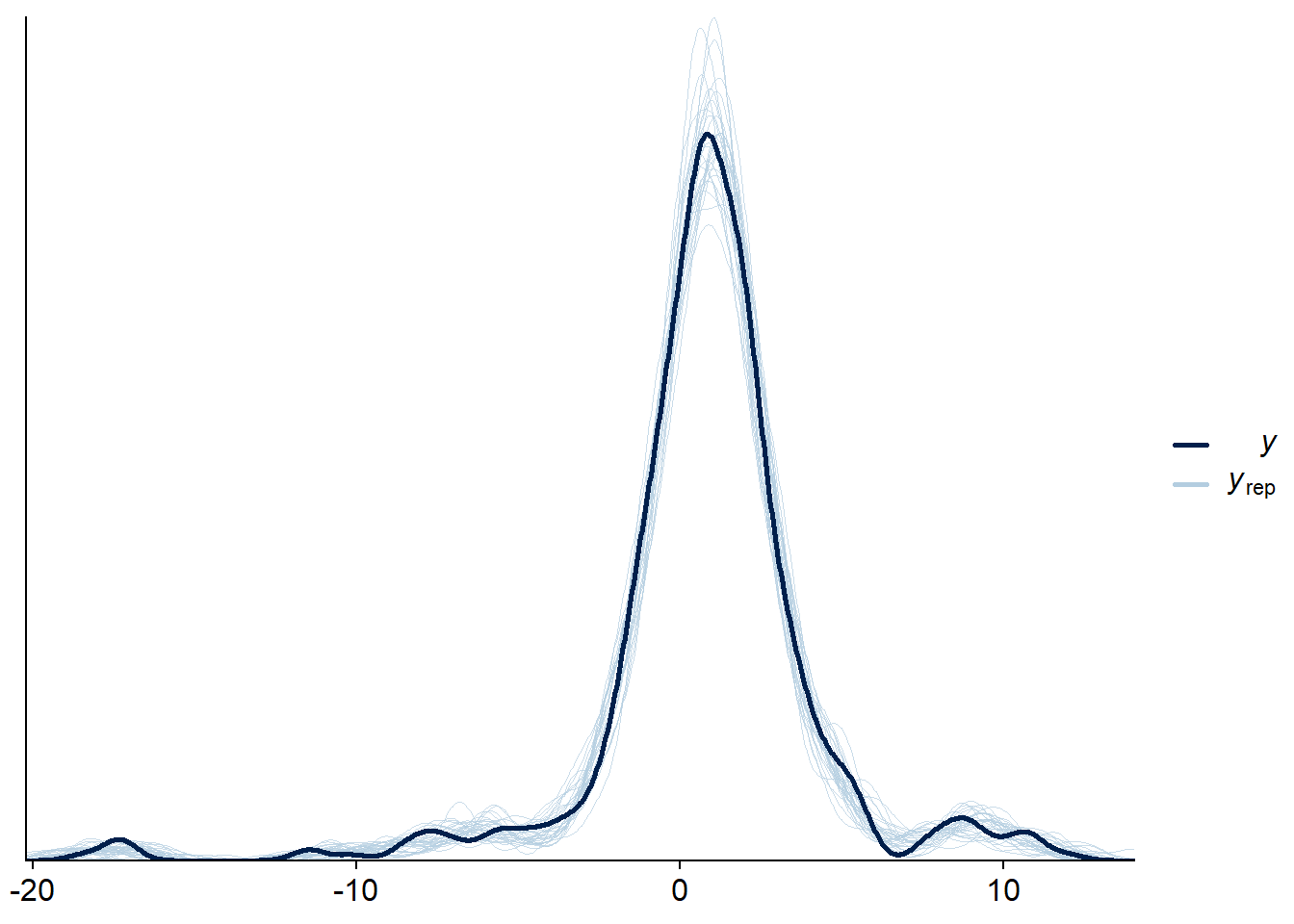

Summary

So yay, we can use brms for the core of our model and then extend it to cover predictors for the standard deviation of random effects. Unfortunately, it requires quite a bit of extra work. Using this heavy machinery for such a simple model as we did in this quick example is probably an overkill and you would be better off just implementing the whole thing in Stan. But if your current brms model is quite complex and the only extra thing you need are the sd predictors, then the cost-benefit considerations might be quite different.

The techniques we used to hack around brms are also very general, note that we have shown how to:

• Combine multiple datasets of different sizes/shapes in a single model
• Replace likelihood with arbitrary Stan code

Together this is enough to use brms-style predictors in connection with basically any type of model. For example, these tricks power my implementation of hidden Markov models with brms discussed at https://discourse.mc-stan.org/t/fitting-hmms-with-time-varying-transition-matrices-using-brms-a-prototype/19645/7 .

Appendix: Check with SBC

Recovering parameters from a single simulation and a nice posterior predictive check are good starting points but far from a guarantee that we implemented the model correctly. To be sure, we’ll check with SBC — if you are not familiar, SBC is a method that can discover almost all implementation problems in your model by repeatedly fitting simulated data. We’ll use the SBC R package and won’t explain all the details here — check the Getting started and SBC for brms vignettes for explanation of the main concepts and API.

# Setting up SBC and paralellism
library(SBC)
future::plan(future::multisession)
gamma_shape <- 14
gamma_rate <- 4
trt_intercept_prior_mu <- 0.5
trt_intercept_prior_sigma <- 0.5

To make the model work with SBC we add explicit priors for all parameters (as the simulations need to match those priors). We’ll use \(N(0,1)\) for most parameters except the intercept for random effect deviations (\(\alpha^\prime\)) where we’ll use \(N(0.5,0.5)\) to avoid both very low and very large standard deviations which pose convergence problems. Similarly, very low observation sigma causes convergence problems, so we’ll use a \(\Gamma(14, 4)\) prior (roughly saying that a priori the standard deviation is unlikely to be less than 1.9 or more than 5.6 ). I did not investigate deeply to understand the convergence issues, so not completely sure about the mechanism.

get_prior(f, combined_data)

##                   prior     class  coef group resp dpar nlpar lb   ub
##                  (flat)         b                                    
##                  (flat) Intercept                                    
##                  (flat)         b             trty                   
##                  (flat)         b trt_x       trty                   
##    student_t(3, 0, 2.5) Intercept             trty                   
##                  (flat)         b                y                   
##                  (flat)         b     x          y                   
##  student_t(3, 0.9, 2.5) Intercept                y                   
##    student_t(3, 0, 2.5)     sigma                y             0 <NA>
##        source
##       default
##       default
##       default
##  (vectorized)
##       default
##       default
##  (vectorized)
##       default
##       default

priors <- c(
  set_prior("normal(0,1)", class = "b", resp = "trty"),
  set_prior(paste0("normal(",trt_intercept_prior_mu, ", ", 
                   trt_intercept_prior_sigma, ")"), 
            class = "Intercept", resp = "trty"),
  set_prior("normal(0,1)", class = "b", resp = "y"),
  set_prior("normal(0,1)", class = "Intercept", resp = "y"),
  set_prior(paste0("gamma(", gamma_shape, ", ", gamma_rate, ")"), 
            class = "sigma", resp = "y")
)

# Function to generate a single simulated dataset
# Note: we reuse N_trts, N, N_pts, patient_id and patient_treatment 
# from the previous code to keep the data passed via stanvars fixed.
generator_func <- function() {
  trt_intercept <- rnorm(1, mean = trt_intercept_prior_mu, 
                         sd = trt_intercept_prior_sigma)
  trt_x_b <- rnorm(1)

  trt_data <- data.frame(trt_x = rnorm(N_trts))
  # Centering predictors to match brms
  trt_data$trt_x <- trt_data$trt_x - mean(trt_data$trt_x)
  trt_sd <- exp(trt_intercept + trt_x_b * trt_data$trt_x)
  
  ranef_raw <- rnorm(N_pts)
  ranef <- ranef_raw * trt_sd[patient_treatment]
  
  intercept <- rnorm(1)
  x_b <- rnorm(1)
  obs_sigma <- rgamma(1, gamma_shape, gamma_rate)
  
  obs_data <- data.frame(x = rnorm(N), 
                          patient_id = base_data$patient_id)
  
  obs_data$x <- obs_data$x - mean(obs_data$x)
  obs_data$trt_id <- patient_treatment[obs_data$patient_id]
  
  obs_data_predictor <- intercept + x_b * obs_data$x + ranef[obs_data$patient_id]
  obs_data$y <- rnorm(N, mean = obs_data_predictor , sd = obs_sigma)
  
  combined_data <- rbind(
    obs_data %>% mutate(
      is_trt = FALSE,
      trt_x = 0,
      trt_y = 0
    ),
    trt_data %>% mutate(
      is_trt = TRUE,
      trt_id = 0,
      patient_id = 0,
      y = 0,
      x = 0,
      trt_y = 0
    )
  )
  
  list(generated = combined_data,
       variables = list(
         b_y_Intercept = intercept,
         b_y_x = x_b,
         b_trty_Intercept = trt_intercept,
         b_trty_trt_x = trt_x_b,
         sigma_y = obs_sigma,
         my_ranef_raw = ranef_raw
       ))
}

# Generate a lot of datsets
set.seed(33214855)
N_sims <- 1000
ds <- generate_datasets(SBC_generator_function(generator_func), n_sims = N_sims)

# With 1000 datasets, this takes ~45 minutes on my computer
backend <-
  SBC_backend_brms(f,
                   stanvars = predict_ranef_stanvars,
                   prior = priors,
                   template_data = combined_data,
                   chains = 2,
                   out_stan_file = file.path(cache_dir, "backend.stan")
                   )

To increase the power of SBC to detect problems, we will also add the log-likelihood and log-prior as derived quantities (see Modrák et al. 2023 or the limits of SBC vignette for background on this).

compute_loglik <- function(y, is_trt, x, trt_x, patient_id, 
                           trt_id, intercept, x_b, trt_intercept, trt_x_b, 
                           ranef_raw, sigma_y) {
  patient_id <- patient_id[!is_trt]
  trt_id <- trt_id[!is_trt]
  x <- x[!is_trt]
  y <- y[!is_trt]
  
  trt_x <- trt_x[is_trt]
  
  patient_trt_all <- matrix(nrow = length(patient_id), ncol = 2)
  patient_trt_all[,1] <- patient_id
  patient_trt_all[,2] <- trt_id
  patient_trt_all <- unique(patient_trt_all)

  patient_treatment <- integer(max(patient_id))
  patient_treatment[patient_trt_all[, 1]] <- patient_trt_all[, 2]
  
  ranef_sigma <- exp(trt_intercept + trt_x * trt_x_b)
  ranef_vals <- ranef_raw * ranef_sigma[patient_treatment]
  mu <- intercept + x * x_b + ranef_vals[patient_id]
  sum(dnorm(y, mean = mu, sd = sigma_y, log = TRUE))  
}


dq <- derived_quantities(
  lprior_fixed = dnorm(b_y_Intercept, log = TRUE) +
    dnorm(b_y_x, log = TRUE) +
    dnorm(b_trty_Intercept, mean = trt_intercept_prior_mu, 
          sd = trt_intercept_prior_sigma, log = TRUE) +
    dnorm(b_trty_trt_x, log = TRUE) +
    dgamma(sigma_y, gamma_shape, gamma_rate, log = TRUE),
  loglik = compute_loglik(y = y, is_trt = is_trt, x = x, trt_x = trt_x,
                          patient_id = patient_id, trt_id = trt_id,
                          intercept = b_y_Intercept, x_b = b_y_x,
                          trt_intercept = b_trty_Intercept, 
                          trt_x_b = b_trty_trt_x, ranef_raw = my_ranef_raw,
                          sigma = sigma_y),
  .globals = c("compute_loglik", "gamma_shape", "gamma_rate",
               "trt_intercept_prior_mu", "trt_intercept_prior_sigma")
)

We are now ready to actually run SBC:

sbc_res <-
  compute_SBC(
    ds,
    backend,
    dquants = dq,
    cache_mode = "results",
    cache_location = file.path(cache_dir, paste0("sbc", N_sims, ".rds")),
    keep_fits = N_sims <= 50
  )

## Results loaded from cache file 'sbc1000.rds'

##  - 305 (30%) fits had at least one Rhat > 1.01. Largest Rhat was 1.39.

##  - 2 (0%) fits had tail ESS undefined or less than half of the maximum rank, potentially skewing 
## the rank statistics. The lowest tail ESS was 13.
##  If the fits look good otherwise, increasing `thin_ranks` (via recompute_SBC_statistics) 
## or number of posterior draws (by refitting) might help.

##  - 2 (0%) fits had divergent transitions. Maximum number of divergences was 2.

##  - 11 (1%) fits had iterations that saturated max treedepth. Maximum number of max treedepth was 2000.

##  - 999 (100%) fits had some steps rejected. Maximum number of rejections was 29.

## Not all diagnostics are OK.
## You can learn more by inspecting $default_diagnostics, $backend_diagnostics 
## and/or investigating $outputs/$messages/$warnings for detailed output from the backend.

There are still some convergence problems for some fits — the most worrying are the high Rhats, affecting almost a third of the fits. This should definitely warrant some further investigation, but the Rhats are not very large and this is a blog post, not a research paper, so we will not go down this rabbit hole.

A very small number of fits had divergences/treedepth issues, but due to the small number, those are not so worrying. The steps rejected is completely benign as this includes rejections during warmup.

Overall, it is in fact safe to just ignore the problematic fits as long as you would not use results from such fits in actual practice (which you shouldn’t) — see the rejection sampling vignette for more details.

We plot the results of the ECDF diff check — looking good!

vars <- sbc_res$stats %>% filter(!grepl("my_", variable)) %>% 
  pull(variable) %>% unique() %>% c("my_ranef_raw[1]", "my_ranef_raw[2]")

excluded_fits <- sbc_res$backend_diagnostics$n_divergent > 0 |
  sbc_res$backend_diagnostics$n_max_treedepth > 0 |
  sbc_res$default_diagnostics$min_ess_tail < 200 |
  sbc_res$default_diagnostics$max_rhat > 1.01
sbc_res_filtered <- sbc_res[!excluded_fits]
plot_ecdf_diff(sbc_res_filtered, variables = vars)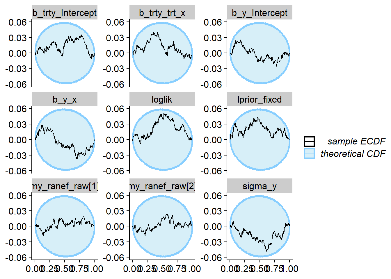

We can also see how close to the true values our estimates are — once again this looks quite good — we do learn quite a lot of information about all parameters except for the random effects!

plot_sim_estimated(sbc_res_filtered, variables = vars, alpha = 0.1)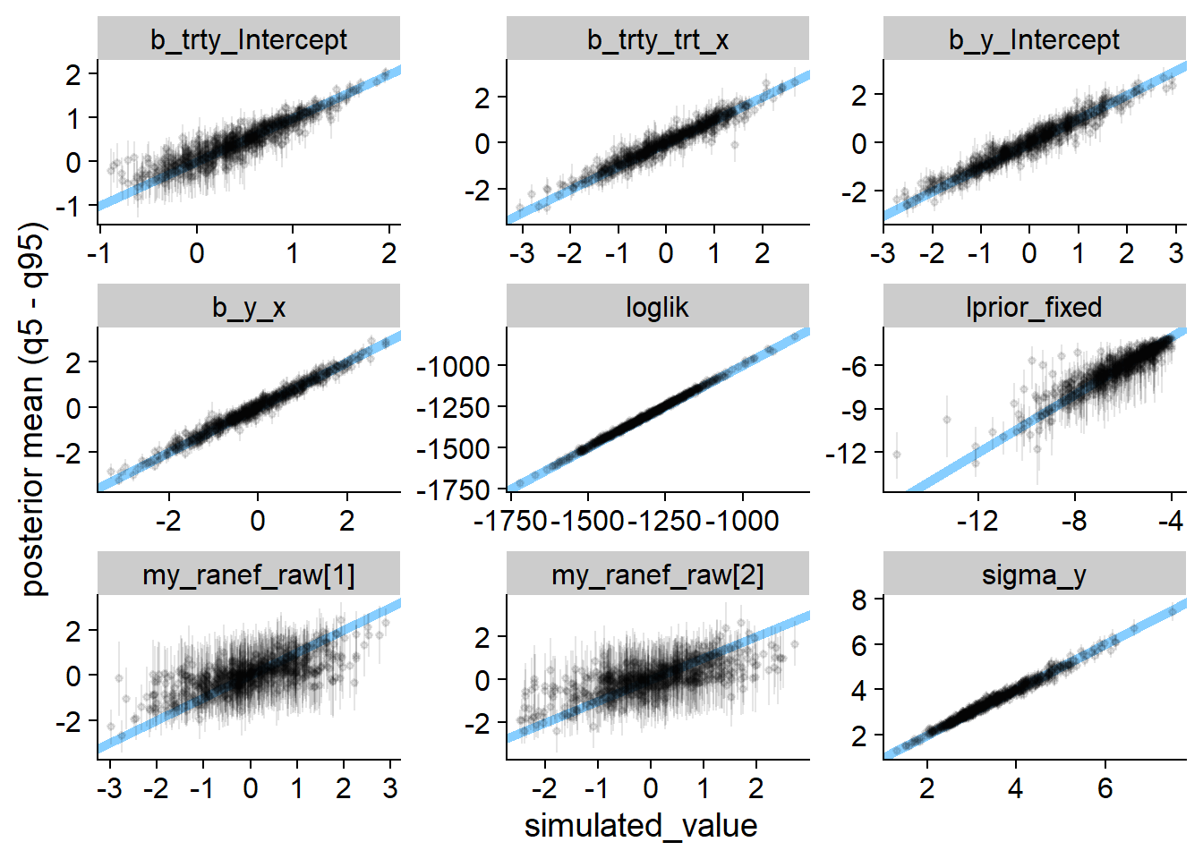

And that’s all. If you encounter problems running the models that you can’t resolve yourself, be sure to ask questions on Stan Discourse and tag me (@martinmodrak) in the question!

Original computing environment

This post was built from Git revision c9ed4bf49cb0082db9ad33f42c00c964d158c3f9, you can download the renv.lock file required to reconstruct the environment.

sessionInfo()

## R version 4.3.2 (2023-10-31 ucrt)
## Platform: x86_64-w64-mingw32/x64 (64-bit)
## Running under: Windows 10 x64 (build 19045)
## 
## Matrix products: default
## 
## 
## locale:
## [1] LC_COLLATE=Czech_Czechia.utf8  LC_CTYPE=Czech_Czechia.utf8   
## [3] LC_MONETARY=Czech_Czechia.utf8 LC_NUMERIC=C                  
## [5] LC_TIME=Czech_Czechia.utf8    
## 
## time zone: Europe/Prague
## tzcode source: internal
## 
## attached base packages:
## [1] stats     graphics  grDevices datasets  utils     methods   base     
## 
## other attached packages:
##  [1] SBC_0.2.0.9000   bayesplot_1.11.1 knitr_1.45       lubridate_1.9.3 
##  [5] forcats_1.0.0    stringr_1.5.1    dplyr_1.1.4      purrr_1.0.2     
##  [9] readr_2.1.5      tidyr_1.3.1      tibble_3.2.1     ggplot2_3.4.4   
## [13] tidyverse_2.0.0  brms_2.20.4      Rcpp_1.0.12      cmdstanr_0.7.1  
## 
## loaded via a namespace (and not attached):
##   [1] gridExtra_2.3        inline_0.3.19        rlang_1.1.3         
##   [4] magrittr_2.0.3       matrixStats_1.2.0    compiler_4.3.2      
##   [7] loo_2.6.0            vctrs_0.6.5          reshape2_1.4.4      
##  [10] pkgconfig_2.0.3      fastmap_1.1.1        backports_1.4.1     
##  [13] ellipsis_0.3.2       labeling_0.4.3       utf8_1.2.4          
##  [16] threejs_0.3.3        promises_1.2.1       rmarkdown_2.25      
##  [19] tzdb_0.4.0           markdown_1.12        ps_1.7.6            
##  [22] xfun_0.42            cachem_1.0.8         jsonlite_1.8.8      
##  [25] highr_0.10           later_1.3.2          parallel_4.3.2      
##  [28] R6_2.5.1             dygraphs_1.1.1.6     bslib_0.6.1         
##  [31] stringi_1.8.3        StanHeaders_2.32.5   parallelly_1.37.0   
##  [34] jquerylib_0.1.4      bookdown_0.37        rstan_2.32.5        
##  [37] zoo_1.8-12           base64enc_0.1-3      timechange_0.3.0    
##  [40] httpuv_1.6.14        Matrix_1.6-1.1       igraph_2.0.1.1      
##  [43] tidyselect_1.2.0     rstudioapi_0.15.0    abind_1.4-5         
##  [46] yaml_2.3.8           codetools_0.2-19     miniUI_0.1.1.1      
##  [49] blogdown_1.19        processx_3.8.3       listenv_0.9.1       
##  [52] pkgbuild_1.4.3       lattice_0.21-9       plyr_1.8.9          
##  [55] shiny_1.8.0          withr_3.0.0          bridgesampling_1.1-2
##  [58] posterior_1.5.0      coda_0.19-4.1        evaluate_0.23       
##  [61] future_1.33.1        RcppParallel_5.1.7   xts_0.13.2          
##  [64] pillar_1.9.0         tensorA_0.36.2.1     checkmate_2.3.1     
##  [67] renv_1.0.2           DT_0.31              stats4_4.3.2        
##  [70] shinyjs_2.1.0        distributional_0.4.0 generics_0.1.3      
##  [73] hms_1.1.3            rstantools_2.4.0     munsell_0.5.0       
##  [76] scales_1.3.0         globals_0.16.2       gtools_3.9.5        
##  [79] xtable_1.8-4         glue_1.7.0           tools_4.3.2         
##  [82] shinystan_2.6.0      colourpicker_1.3.0   mvtnorm_1.2-4       
##  [85] cowplot_1.1.3        grid_4.3.2           QuickJSR_1.1.3      
##  [88] crosstalk_1.2.1      colorspace_2.1-0     nlme_3.1-163        
##  [91] cli_3.6.2            fansi_1.0.6          Brobdingnag_1.2-9   
##  [94] gtable_0.3.4         sass_0.4.8           digest_0.6.34       
##  [97] farver_2.1.1         htmlwidgets_1.6.4    memoise_2.0.1       
## [100] htmltools_0.5.7      lifecycle_1.0.4      mime_0.12           
## [103] shinythemes_1.2.0