Although my time with the Stan language has been enjoyable, there is one thing that is not fun when modelling with Stan. And it is the dreaded warning message:
There were X divergent transitions after warmup.
Increasing adapt_delta above 0.8 may help.
Now once you have increased adapt_delta to no avail, what should you do? Divergences (and max-treedepth and low E-BFMI warnings alike) tell you there is something wrong with your model, but do not exactly tell you what. There are numerous tricks and strategies to diagnose convergence problems, but currently, those are scattered across Stan documentation, Discourse and the old mailing list. Here, I will try to bring all the tricks that helped me at some point to one place for the reference of future desperate modellers.
The strategies
This list is outdated, the Guide to Stan warnings has a better list of debugging hints.
I don’t want to keep you waiting, so below is a list of all strategies I have ever used to diagnose and/or remedy divergences:
Check your code. Twice. Divergences are almost as likely a result of a programming error as they are a truly statistical issue. Do all parameters have a prior? Do your array indices and for loops match?
Create a simulated dataset with known true values of all parameters. It is useful for so many things (including checking for coding errors). If the errors disappear on simulated data, your model may be a bad fit for the actual observed data.
Check your priors. If the model is sampling heavily in the very tails of your priors or on the boundaries of parameter constraints, this is a bad sign.
Visualisations: use
mcmc_parcoordfrom thebayesplotpackage, Shinystan andpairsfromrstan. Documentation for Stan Warnings (contains a few hints), Case study - diagnosing a multilevel model, Gabry et al. 2017 - Visualization in Bayesian workflowMake sure your model is identifiable - non-identifiability and/or multimodality (multiple local maxima of the posterior distributions) is a problem. Case study - mixture models, my post on non-identifiable models and how to spot them.
Run Stan with the
test_gradoption.Reparametrize your model to make your parameters independent (uncorrelated) and close to N(0,1) (a.k.a change the actual parameters and compute your parameters of interest in the
transformed parametersblock).Try non-centered parametrization - this is a special case of reparametrization that is so frequently useful that it deserves its own bullet. Case study - diagnosing a multilevel model, Betancourt & Girolami 2015
Move parameters to the
datablock and set them to their true values (from simulated data). Then return them one by one toparemtersblock. Which parameter introduces the problems?Introduce tight priors centered at true parameter values. How tight need the priors to be to let the model fit? Useful for identifying multimodality.
Play a bit more with
adapt_delta,stepsizeandmax_treedepth. Example
In the coming weeks I hope to be able to provide separate posts on some of the bullets above with a worked-out example. In this introductory post I will try to provide you with some geometric intuition behind what divergences are.
Before We Delve In
Caveat: I am not a statistician and my understanding of Stan, the NUTS sampler and other technicalities is limited, so I might be wrong in some of my assertions. Please correct me, if you find mistakes.
Make sure to follow Stan Best practices. Especially, start with a simple model, make sure it works and add complexity step by step. I really cannot repeat this enough. To be honest, I often don’t follow this advice myself, because just writing the full model down is so much fun. To be more honest, this has always resulted in me being sad and a lots of wasted time.
Also note that directly translating models from JAGS/BUGS often fails as Stan requires different modelling approaches. Stan developers have experienced first hand that some JAGS models produce wrong results and do not converge even in JAGS, but no one noticed before they compared their output to results from Stan.
What Is a Divergence?
Following the Stan manual:
A divergence arises when the simulated Hamiltonian trajectory departs from the true trajectory as measured by departure of the Hamiltonian value from its initial value.
What does that actually mean? Hamiltonian is a function of the posterior density and auxiliary momentum parameters. The auxiliary parameters are well-behaved by construction, so the problem is almost invariably in the posterior density. Keep in mind that for numerical reasons Stan works with the logarithm of posterior density (also known as: log_prob, __lp and target). The NUTS sampler performs several discrete steps per iteration and is guided by the gradient of the density. With some simplification, the sampler assumes that the log density is approximately linear at the current point, i.e. that small change in parameters will result in small change in log-density. This assumption is approximately correct if the step size is small enough. Lets look at two different step sizes in a one-dimensional example:
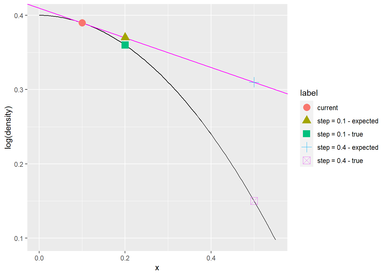 The sampler starts at the red dot, the black line is the log-density, magenta line is the gradient. When moving 0.1 to the right, the sampler expects the log-density to decrease linearly (green triangle) and although the actual log-density decreases more (the green square), the difference is small. But when moving 0.4 to the right the difference between expected (blue cross) and actual (pink crossed square) becomes much larger. It is a large discrepancy of a similar kind that is signalled as a divergence. During warmup Stan will try to adjust the step size to be small enough for divergences to not occur, but large enough for the sampling to be efficient. But if the parameter space is not well behaved, this might not be possible. Why? Keep on reading, fearless reader.
2D Examples
Lets try to build some geometric intuition in 2D parameter space. Keep in mind that sampling is about exploring the parameter space proportionally to the associated posterior density - or, in other words - exploring uniformly across the volume between the zero plane and the surface defined by density (probability mass). For simplicity, we will ignore the log transform Stan actually doeas and talk directly about density in the rest of this post. Imagine the posterior density is a smooth wide hill:
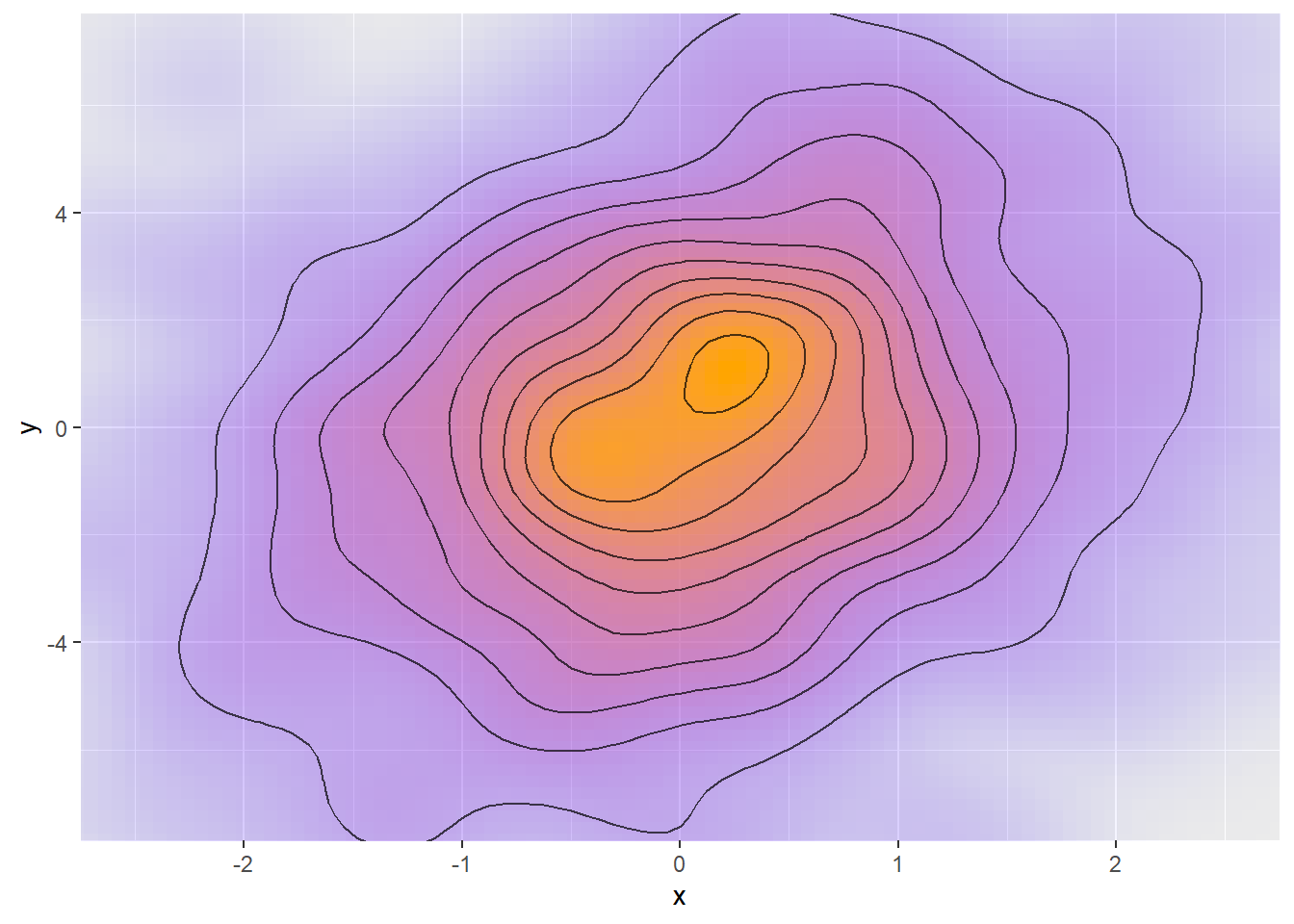
Stan starts each iteration by moving across the posterior in random direction and then lets the density gradient steer the movement preferrentially to areas with high density. To explore the hill efficiently, we need to take quite large steps in this process - the chain of samples will represent the posterior well if it can move across the whole posterior in a small-ish number of steps (actually at most 2^max_treedepth steps). So average step size of something like 0.1 might be reasonable here as the posterior is approximately linear at this scale. We need to spend a bit more time around the center, but not that much, as there is a lot of volume also close to the edges - it has lower density, but it is a larger area.
Now imagine that the posterior is much sharper:
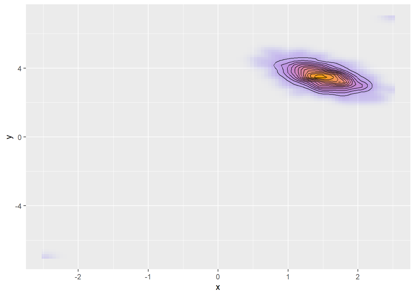 Now we need much smaller steps to explore safely. Step size of 0.1 won’t work as the posterior is non-linear on this scale, which will result in divergences. The sampler is however able to adapt and chooses a smaller step size accordingly. Another thing Stan will do is to rescale dimensions where the posterior is narrow. In the example above, posterior is narrower in
 y and thus this dimension will be inflated to roughly match the spread in x. Keep in mind that Stan rescales each dimension separately (the posterior is transformed by a diagonal matrix).
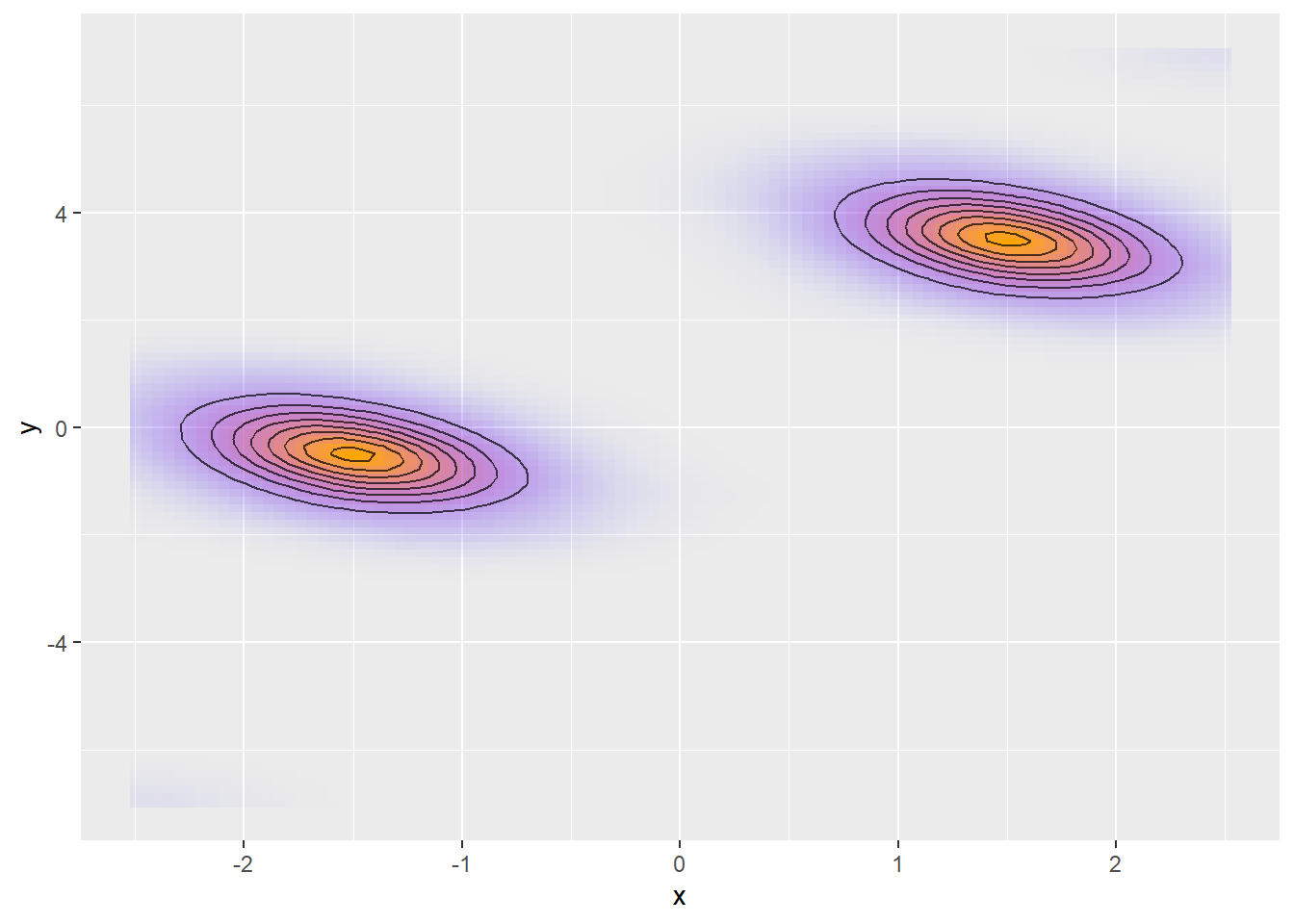
Now what if the posterior is a combination of both a “smooth hill” and a “sharp mountain”?
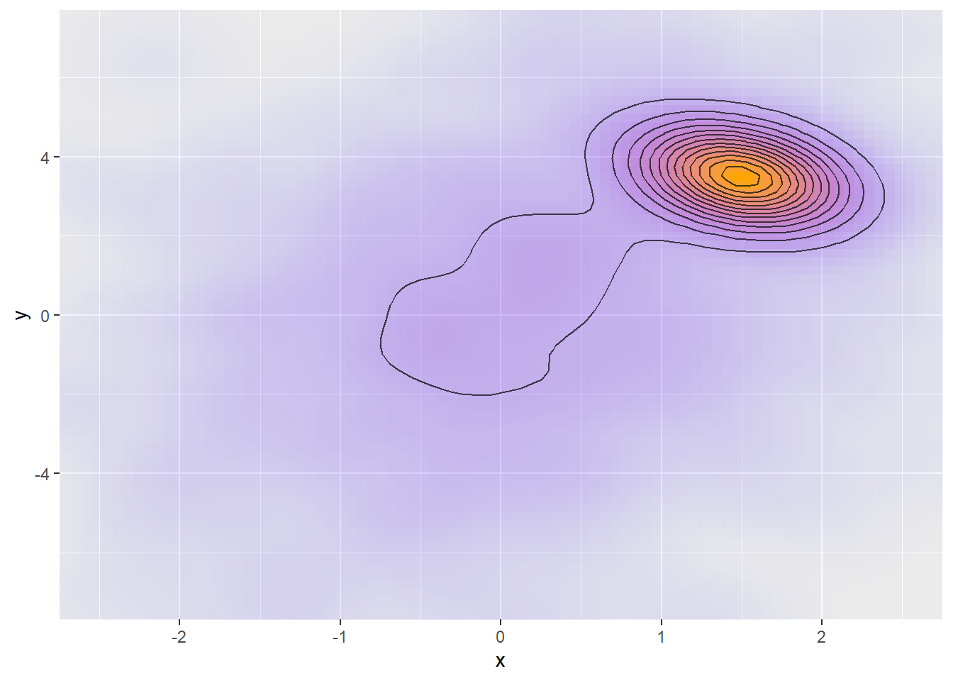 The sampler should spend about half the time in the “sharp mountain” and the other half in the “smooth hill”, but those regions need different step sizes and the sampler only takes one step size. There is also no way to rescale the dimensions to compensate. A chain that adapted to the “smooth hill” region will experience divergences in the “sharp mountain” region, a chain that adapted to the “sharp mountain” will not move efficiently in the “smooth hill” region (which will be signalled as transitions exceeding maximum treedepth). The latter case is however less likely, as the “smooth hill” is larger and chains are more likely to start there. I think that this is why problems of this kind mostly manifest as divergences and less likely as exceeding maximum treedepth.
This is only one of many reasons why multimodal posterior hurts sampling. Multimodality is problematic even if all modes are similar - one of the other problems is that traversing between modes might require much larger step size than exploration within each mode, as in this example:
I bet Stan devs would add tons of other reasons why multimodality is bad for you (it really is), but I’ll stop here and move to other possible sources of divergences.
The posterior geometry may be problematic, even if it is unimodal. A typical example is a funnel, which often arises in multi-level models:
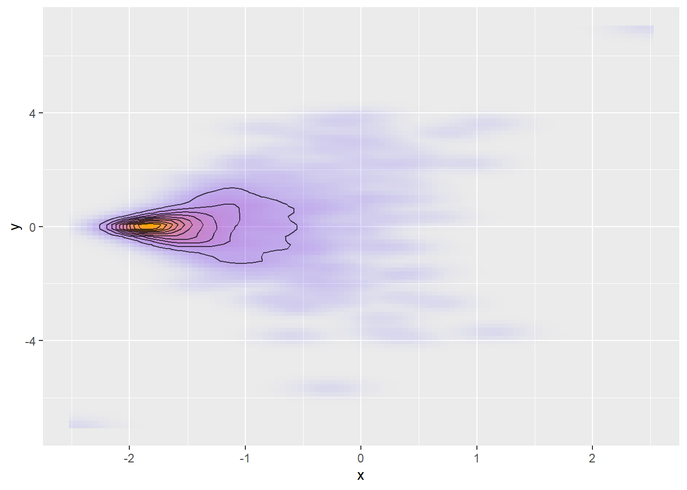 Here, the sampler should spend a lot of time near the peak (where it needs small steps), but a non-negligible volume is also found in the relatively low-density but large area on the right where a larger step size is required. Once again, there is no way to rescale each dimension independently to selectively “stretch” the area around the peak. Similar problems also arise with large regions of constant or almost constant density combined with a single mode.
Last, but not least, lets look at tight correlation between variables, which is a different but frequent problem:
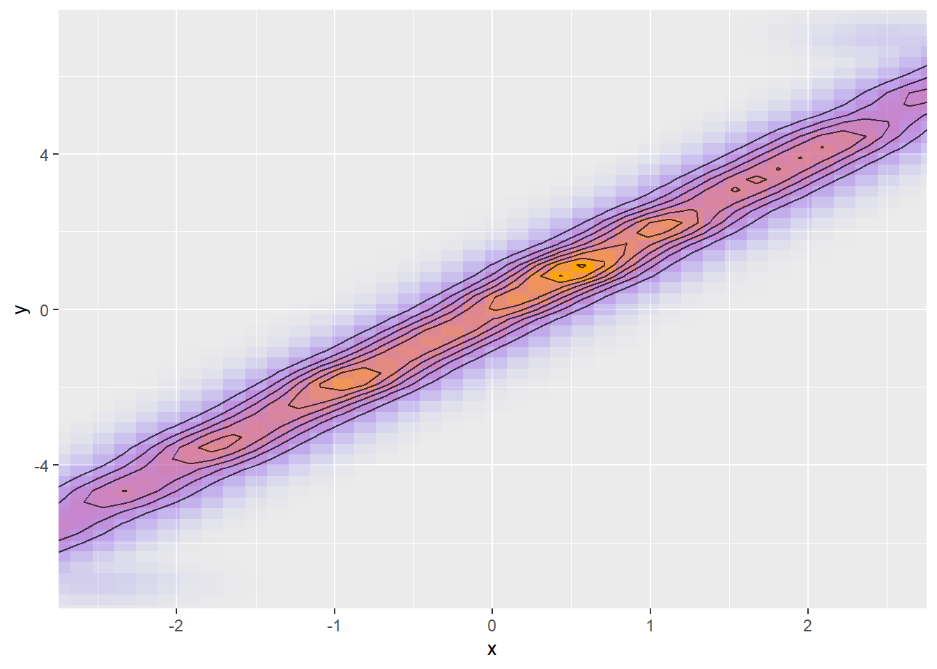 The problem is that if we are moving in the direction of the ridge, we need large step size, but when we move tangentially to that direction, we need small step size. Once again, Stan is unable to rescale the posterior to compensate as scaling
 x or y on its own will increase both width and length of the ridge.
Things get even more insidious when the relationship between the two variables is not linear:
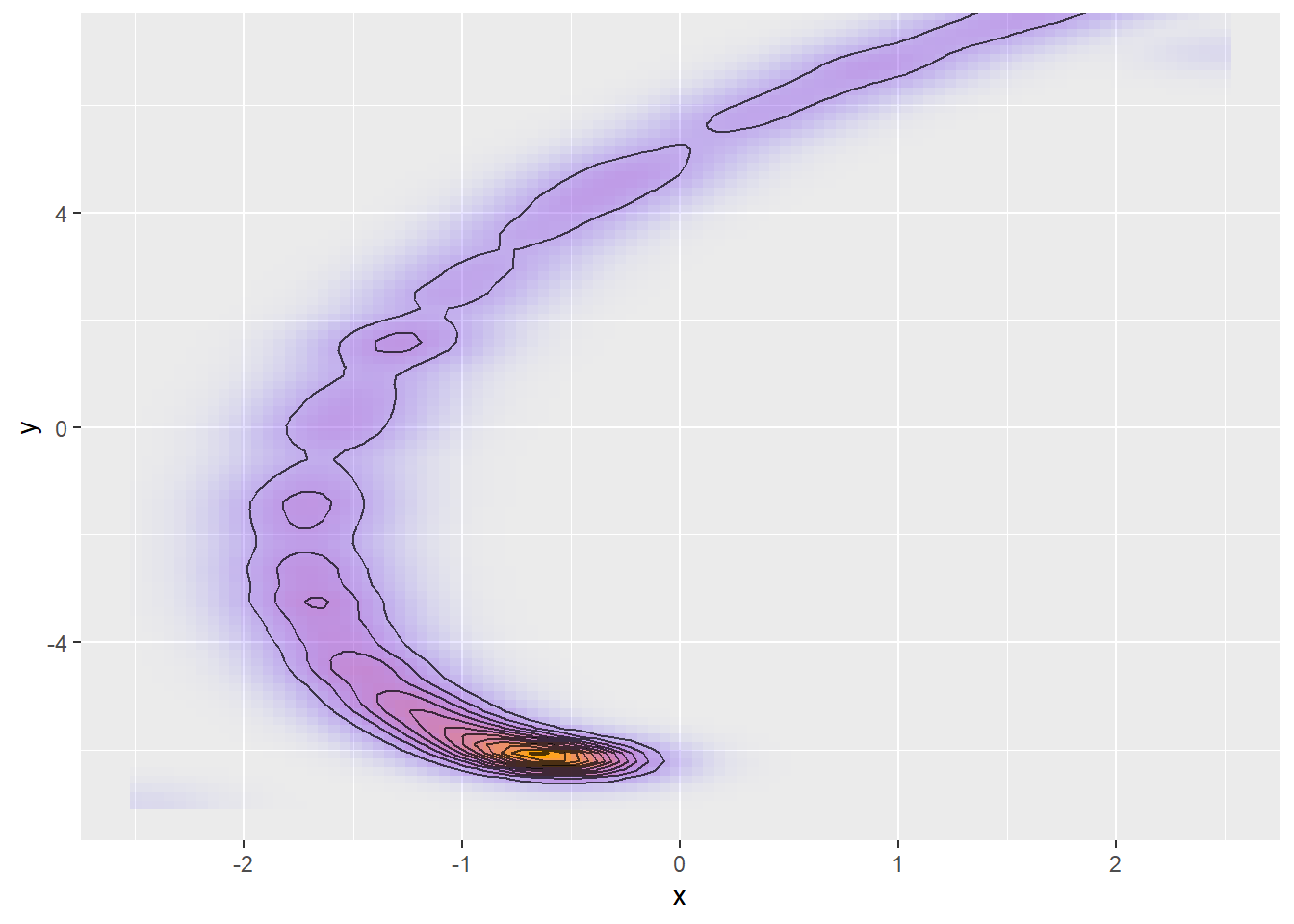
Here, a good step size is a function of both location (smaller near the peak) and direction (larger when following the spiral) making this kind of posterior hard to sample.
Bigger Picture
This has been all pretty vague and folksy. Remeber these examples are there just to provide intuition. To be 100% correct, you need to go to the NUTS paper and/or the Conceptual Introduction to HMC paper and delve in the math. The math is always correct.
In particular all the above geometries may be difficult for NUTS and seeing them in visualisations hints at possible issues, but they may also be handled just fine. In fact, I wouldn’t be surprised if Stan worked with almost anything in two dimensions. Weak linear correlations that form wide ridges are also - in my experience - quite likely to be sampled well, even in higher dimensions. The issues arise when regions of non-negligible density are very narrow in some directions and much wider in others and rescaling each dimension individually won’t help. And finally, keep in mind that the posterios we discussed are even more difficult for Gibbs or other older samplers - and Gibbs will not even let you know there was a problem.
Love Thy Divergences
The amazing thing about divergences is that what is essentially a numerical problem actually signals a wide array of possibly severe modelling problems. Be glad - few algorithms (in any area) have such a clear signal that things went wrong. This is also the reason why you should be suspicious about your results even when only a single divergence had been reported - you don’t know what is hiding in the parts of your posterior that are inaccessible with the current step size.
That’s all for now. Hope to see you in the future with examples of actual diverging Stan models.