This is a second post in my series on taming divergences in Stan models, see the first post in the series for a general introduction. Also see guide to Stan warnings
Standard caveat: I am not an expert on Stan, I consider myself just an advanced user who likes to explain things. Please point out any errors, things that contradict your experience or anything else you do not trust.
What is “non-identifiability”
In a strict sense, it means that two values of the parameters result in the same probability distribution of observed data. It is also sometimes used to cover situations when there is not a unique local maximum of the posterior density - either because there are multiple separate maxima or because there is ridge/plateau where a set of points has the same posterior density (those may or may not be identifiable in the strict sense).
On the Stan forums the term seems to be used in even a bit broader sense and also covers cases where the maximum of the posterior density is in a region that is approximately flat. This often happens when the posterior is dominated by the prior and the likelihood provides little information about the parameters. If this is the case, it is sometimes said that the model is weakly identified. A weakly identified model may become non-identified in the strict sense if a prior is not specified for all parameters. This is just another reason to specify proper priors for everything.
Problems with identifiability are just one class of issues that are signalled in Stan by divergences and/or other diagnostics (max treedepth, low BFMI, low n_eff, large Rhat), the first post in this series has a more extensive list of other possible causes. Note also that except for Stan, most statistical/ML software won’t complain when you try to fit non-identifiable models, even though it may lead to noticeably biased inferences.
Scope
In this post I will show a few different types of issues that result from limited identifiability. I will also try to show how to spot these problems in various visualisations. Remember that instead of creating the plots in code as we do here, you can use ShinyStan to explore many visualisations interactively.
We will start with some weakly identified non-linear regression models and move toward models that are hopelessly multimodal (have multiple local maxima of posterior density), including a small neural network and Gaussian process with a Berkson-style error. I will focus on models that don’t have any obvious error (like ommitted prior), although such errors can lead to non-identifiability. A recurring theme in this post is that identifiability may depend on the actual data as well as the model, keep that in mind when modelling!
A frequent source of fitting issues due to non-identifiability are mixture models. There is an excellent case study for mixture models by Michael Betancourt and I have nothing to add to this topic, so mixtures are not covered here.
The post got pretty long so let’s not hesitate and get our hands dirty!
library(tidyverse)
library(rstan)
library(bayesplot)
library(tidybayes)
library(knitr)
library(here)
library(rgl)
knit_hooks$set(webgl = hook_webgl)
theme_set(cowplot::theme_cowplot())

rstan_options(auto_write = TRUE)
options(mc.cores = parallel::detectCores())
A weakly-identified linear model that (mostly) works
First, let’s start with a model I thought would have problems but that ended up mostly OK. The model is a simple regression with a quadratic term:
\[ \begin{align} \mu_i &= \beta_1 x_i + \beta_2 x_i^2 \\ y_i &\sim N(\mu_i, \sigma) \end{align} \] and here is the Stan code:
stan_code_linear <- "
data {
  int N;
  vector[N] y;
  vector[N] x;
  real<lower=0> sigma;
  real<lower=0> prior_width;
}

parameters {
  real beta[2];
}

model {
  y ~ normal(beta[1] * x + beta[2] * square(x), sigma);
  sigma ~ normal(0,1);
  beta ~ normal(0,prior_width);
}
"

model_linear <- stan_model(model_code = stan_code_linear)
When wide array of \(x\) values is available, this model works without any trouble. But what happens when all \(x_i \in \{0,1\}\)? In this case the likelihood cannot distinguish between the contribution of \(\beta_1\) and \(\beta_2\). Let’s simulate some data and have a look at the pairs plot:
set.seed(20180512)

sigma = 1
x = rep(c(0,1), times = 10)
data_linear <- list(
  N = length(x),
  x = x,
  y = rnorm(length(x), x + x ^ 2, sigma),
  sigma = sigma,
  prior_width = 10
)

fit_linear <- sampling(model_linear, data = data_linear)
pairs(fit_linear, pars = "beta")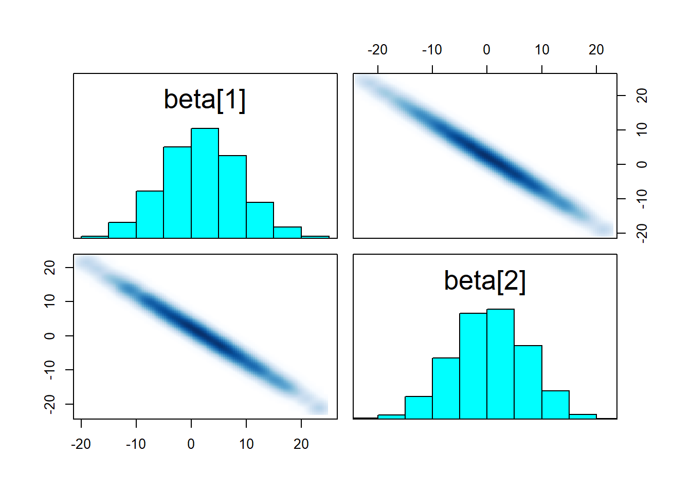
While the result is not very useful, the sampler worked well! We gained little information about each \(\beta\) individually (their range spans alomost all of the prior), but their sum is tightly constrained as witnessed by the strong negative correlation. So what if we increase prior_width to make the prior resemble a flat prior? We do get max treedepth warnings!
set.seed(21645465)

data_linear2 <- data_linear
data_linear2$prior_width = 100
fit_linear2 <- sampling(model_linear, data = data_linear2)
## Warning: There were 263 transitions after warmup that exceeded the maximum treedepth. Increase max_treedepth above 10. See
## https://mc-stan.org/misc/warnings.html#maximum-treedepth-exceeded## Warning: Examine the pairs() plot to diagnose sampling problemspairs(fit_linear2, pars = "beta")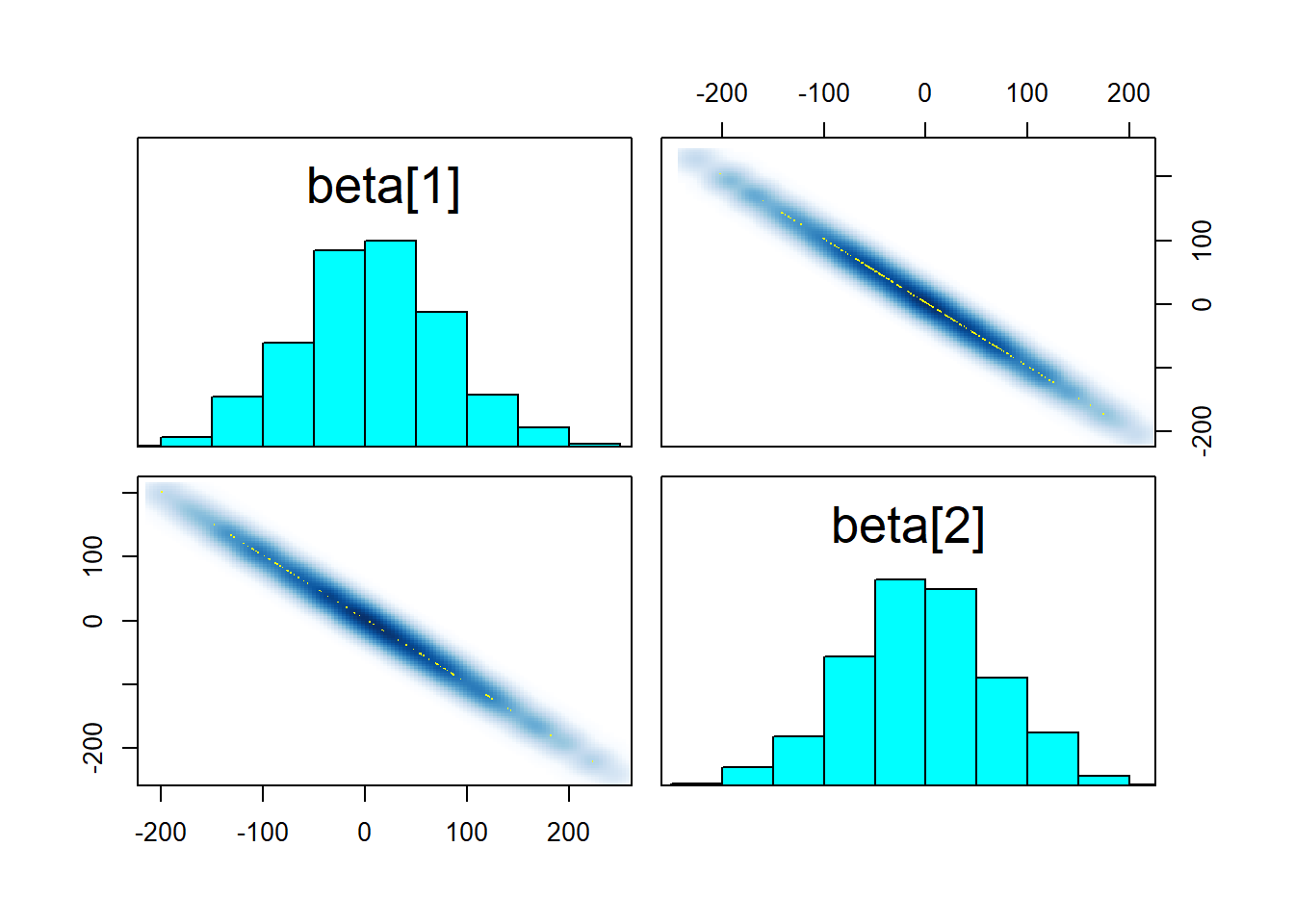
What seems to happen is that the ridge in the posterior becomes too long and the sampler cannot traverse it efficiently, resulting in transitions that exceed the maximum treedepth. The root of the problem is that the sampler has to choose a step size that is shorter than the width of the ridge to not diverge when moving tangentially to the ridge direction. With such a small step size, the sampler cannot move across the length of the ridge in one iteration. Still, the results should be unbiased and if we manage to get a reasonable n_eff (which we do), there is no reason to worry. Improper flat prior would however lead to some actual trouble. Don’t use improper priors, folks!
Take home message: While this particular model works well unless we set the prior too wide, linear correlations in the pairs plot are a bad sign and you should try to avoid them as they can produce problems when interacting with other components of a larger model. It might make sense to reparametrize using the sum or ratio of the variables in question.
A weakly-identified sigmoid model
Let’s move to a model where the non-identifiability actually wreaks havoc. Once again, the model works for some data, but breaks for others - even if all model assumptions do hold. The model tries to determine parameters of a sigmoid function that is observed noisily:
\[ \begin{align} y_{true} &= \frac{1}{1 + e^{-wx-b}} \\ y &\sim N(y_{true},\sigma) \end{align} \]
Here \(w\) and \(b\) are the only parameters of the model. The model is a bit artificial, but it is actually a component of larger gene expression models I work with. The corresponding Stan code is below:
stan_code_sigmoid <- "
data {
  int N;
  vector[N] y;
  vector[N] x;
  real<lower=0> prior_width;
  real<lower=0> sigma;
}

parameters {
  real w;
  real b;
}

model {
  vector[N] y_true = inv_logit(w * x + b);
  y ~ normal(y_true, sigma);
  w ~ normal(0,prior_width);
  b ~ normal(0,prior_width);
}
"

model_sigmoid <- stan_model(model_code = stan_code_sigmoid)
Now lets fit the model to simulated datasets with the exact same true parameter values \(w = b = 1\), but different values of the independent variable \(x\). In the first case, \(x\) is drawn from \(N(0,2)\):
set.seed(214575878)

simulate_sigmoid <- function(x) {
  sigma = 0.1
  w = 1
  b = 1
  N = length(x)
  y_true = 1 / (1 + exp(-w*x-b))
  prior_width = 10

  list(
    N = N,
    x = x,
    y = rnorm(N, y_true, sigma),
    prior_width = prior_width,
    sigma = sigma
  )
}

data_sigmoid_ok <- simulate_sigmoid(rnorm(20, 0, 2))
fit_sigmoid_ok <- sampling(model_sigmoid, data = data_sigmoid_ok)
print(fit_sigmoid_ok)
## Inference for Stan model: anon_model.
## 4 chains, each with iter=2000; warmup=1000; thin=1;
## post-warmup draws per chain=1000, total post-warmup draws=4000.
##
## mean se_mean sd 2.5% 25% 50% 75% 97.5% n_eff Rhat
## w 1.02 0.00 0.14 0.78 0.93 1.01 1.11 1.31 1295 1
## b 1.12 0.00 0.19 0.79 0.99 1.10 1.23 1.51 1404 1
## lp__ -14.66 0.03 1.06 -17.48 -15.07 -14.33 -13.91 -13.66 1318 1
##
## Samples were drawn using NUTS(diag_e) at Sat May 14 13:26:16 2022.
## For each parameter, n_eff is a crude measure of effective sample size,
## and Rhat is the potential scale reduction factor on split chains (at
## convergence, Rhat=1).pairs(fit_sigmoid_ok, pars = c("w","b"))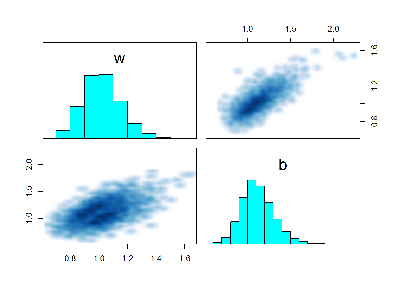
For the first dataset, the model converges and recovers parameters correctly. The pairs plot shows a nice gaussian blob, nothing to worry about. Now let’s try a second dataset, this time \(x\) is drawn from \(N(5,2)\).
data_sigmoid_divergent <- simulate_sigmoid(rnorm(20, 5, 2))
fit_sigmoid_divergent <- sampling(model_sigmoid, data = data_sigmoid_divergent)
## Warning: There were 281 divergent transitions after warmup. See
## https://mc-stan.org/misc/warnings.html#divergent-transitions-after-warmup
## to find out why this is a problem and how to eliminate them.## Warning: Examine the pairs() plot to diagnose sampling problems## Warning: The largest R-hat is 1.06, indicating chains have not mixed.
## Running the chains for more iterations may help. See
## https://mc-stan.org/misc/warnings.html#r-hat## Warning: Bulk Effective Samples Size (ESS) is too low, indicating posterior means and medians may be unreliable.
## Running the chains for more iterations may help. See
## https://mc-stan.org/misc/warnings.html#bulk-ess## Warning: Tail Effective Samples Size (ESS) is too low, indicating posterior variances and tail quantiles may be unreliable.
## Running the chains for more iterations may help. See
## https://mc-stan.org/misc/warnings.html#tail-essprint(fit_sigmoid_divergent)## Inference for Stan model: anon_model.
## 4 chains, each with iter=2000; warmup=1000; thin=1;
## post-warmup draws per chain=1000, total post-warmup draws=4000.
##
## mean se_mean sd 2.5% 25% 50% 75% 97.5% n_eff Rhat
## w 3.91 0.59 5.55 0.30 0.55 0.93 5.62 19.44 89 1.04
## b 1.82 0.17 1.81 0.36 0.90 1.29 2.14 6.04 108 1.03
## lp__ -10.63 0.29 2.48 -16.30 -12.56 -9.79 -8.44 -7.74 73 1.06
##
## Samples were drawn using NUTS(diag_e) at Sat May 14 13:26:52 2022.
## For each parameter, n_eff is a crude measure of effective sample size,
## and Rhat is the potential scale reduction factor on split chains (at
## convergence, Rhat=1).For the second dataset, there is a huge number of divergences and the parameters are largely uncertain and overestimated. So once again, the model is identifiable in principle, but the extreme data introduce problems.
Let’s try to visualise the posteriors - luckily we only have two parameters, so it is easy to see everything at once!
pairs(fit_sigmoid_divergent, pars = c("w","b"))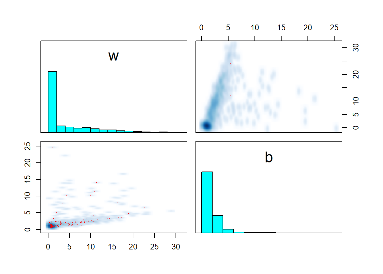
The issue seems to be that for the second dataset, we sampled \(x\) towards the tail of the sigmoid and almost all \(y\) are thus close to 1, giving us little information about the parameters. However, the model strictly enforces that \(w x + b > 0\). This creates a large area of the posterior where the value of \(w\) and \(b\) does not matter much (requiring a large step size to traverse) and a thin sharp boundary around \(wx + b \simeq 0\) where a smaller step size is required to traverse safely. Transitions crossing the boundary often diverge due to large step size and are rejected, leading to overexploration of the flat area and bias.
This is, in my experience, one of the ways that weak identifiability may hurt sampling - the model maybe weakly identified only for a subset of the parameter space while there is another area where the likelihood has a huge contribution and this may require different step size for the sampler.
The issue may be partially redeemed by reparametrization using \(a = \mathrm{E}(wx + b), b = \mathrm{sd}(wx + b)\). You can then set priors on \(a, b\) that avoid the tails of the sigmoid while being independent of \(x\).
Take home message: Sharp boundaries of otherwise diffuse regions in the posterior (as seen above) are worth investigating.
A sigmoid model with non-identified special case
We can make the above model even more problematic by introducing a parameter \(k\) to generalize the sigmoid a bit more:
\[ \begin{align} y_{true} &= \frac{k}{1 + e^{-wx-b}} \\ y &\sim N(y_{true},\sigma) \end{align} \]
giving us the following Stan code:
stan_code_sigmoid2 <- "
data {
  int N;
  vector[N] y;
  vector[N] x;
  real<lower=0> prior_width;
  real<lower=0> sigma;
}

parameters {
  real k;
  real w;
  real b;
}

model {
  vector[N] y_true = k * inv_logit(w * x + b);
  y ~ normal(y_true, sigma);
  w ~ normal(0,prior_width);
  b ~ normal(0,prior_width);
}
"

model_sigmoid2 <- stan_model(model_code = stan_code_sigmoid2)
This time we will simulate two datasets with the same \(x \sim N(0,2)\), avoiding the extreme values. We will set \(k = b = 1\) for both datasets. In addition, the first dataset will have \(w = 1\). Let’s see how that goes:
set.seed(98321456)

simulate_sigmoid2 <- function(x, w) {
  sigma = 0.1
  k = 1
  b = 1
  N = length(x)
  prior_width = 10
  y_true = k / (1 + exp(-w*x-b))

  list(
    N = N,
    x = x,
    y = rnorm(N, y_true, sigma),
    prior_width = prior_width,
    sigma = sigma
  )
}

data_sigmoid2_ok <- simulate_sigmoid2(rnorm(20, 0, 2), w = 1)
fit_sigmoid2_ok <- sampling(model_sigmoid2, data = data_sigmoid2_ok)
print(fit_sigmoid2_ok)
## Inference for Stan model: anon_model.
## 4 chains, each with iter=2000; warmup=1000; thin=1;
## post-warmup draws per chain=1000, total post-warmup draws=4000.
##
## mean se_mean sd 2.5% 25% 50% 75% 97.5% n_eff Rhat
## k 1.05 0.00 0.09 0.90 0.99 1.04 1.11 1.23 1093 1.01
## w 1.08 0.01 0.20 0.75 0.94 1.05 1.20 1.53 1062 1.01
## b 1.06 0.01 0.40 0.38 0.76 1.02 1.31 1.94 1013 1.01
## lp__ -9.06 0.04 1.22 -12.17 -9.65 -8.75 -8.15 -7.63 1210 1.00
##
## Samples were drawn using NUTS(diag_e) at Sat May 14 13:31:14 2022.
## For each parameter, n_eff is a crude measure of effective sample size,
## and Rhat is the potential scale reduction factor on split chains (at
## convergence, Rhat=1).Nice, no problems here. Let’s see what happens when we set \(w = 0\)
data_sigmoid2_divergent <-  simulate_sigmoid2(rnorm(20, 0, 2), w = 0)
fit_sigmoid2_divergent <- sampling(model_sigmoid2, data = data_sigmoid2_divergent)
## Warning: There were 21 divergent transitions after warmup. See
## https://mc-stan.org/misc/warnings.html#divergent-transitions-after-warmup
## to find out why this is a problem and how to eliminate them.## Warning: There were 391 transitions after warmup that exceeded the maximum treedepth. Increase max_treedepth above 10. See
## https://mc-stan.org/misc/warnings.html#maximum-treedepth-exceeded## Warning: Examine the pairs() plot to diagnose sampling problems## Warning: The largest R-hat is 1.57, indicating chains have not mixed.
## Running the chains for more iterations may help. See
## https://mc-stan.org/misc/warnings.html#r-hat## Warning: Bulk Effective Samples Size (ESS) is too low, indicating posterior means and medians may be unreliable.
## Running the chains for more iterations may help. See
## https://mc-stan.org/misc/warnings.html#bulk-ess## Warning: Tail Effective Samples Size (ESS) is too low, indicating posterior variances and tail quantiles may be unreliable.
## Running the chains for more iterations may help. See
## https://mc-stan.org/misc/warnings.html#tail-essprint(fit_sigmoid2_divergent)## Inference for Stan model: anon_model.
## 4 chains, each with iter=2000; warmup=1000; thin=1;
## post-warmup draws per chain=1000, total post-warmup draws=4000.
##
## mean se_mean sd 2.5% 25% 50% 75%
## k 2471033772.87 2.960192e+09 5.236172e+09 0.68 0.72 0.73 15413114.53
## w -0.28 7.000000e-02 1.570000e+00 -4.07 -0.98 0.02 0.41
## b 4.51 1.134000e+01 1.673000e+01 -23.99 -2.97 10.64 15.76
## lp__ -12.38 2.700000e-01 1.240000e+00 -15.46 -13.00 -12.23 -11.43
## 97.5% n_eff Rhat
## k 1.875328e+10 3 2.22
## w 2.770000e+00 471 1.01
## b 2.624000e+01 2 3.46
## lp__ -1.068000e+01 22 1.09
##
## Samples were drawn using NUTS(diag_e) at Sat May 14 13:32:13 2022.
## For each parameter, n_eff is a crude measure of effective sample size,
## and Rhat is the potential scale reduction factor on split chains (at
## convergence, Rhat=1).As has become the habit in this post, the model diverges for the second dataset. Note also that the parameter estimates for \(k\) and \(b\) are way off and their 95% credible intervals exclude the true value! (remember: even a few divergent transitions indicate sampling problems). Let’s have a look at the pair plots for both models:
pairs(fit_sigmoid2_ok, pars = "energy__", include = FALSE)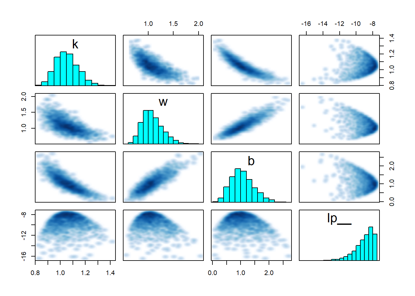
pairs(fit_sigmoid2_divergent, pars = "energy__", include = FALSE)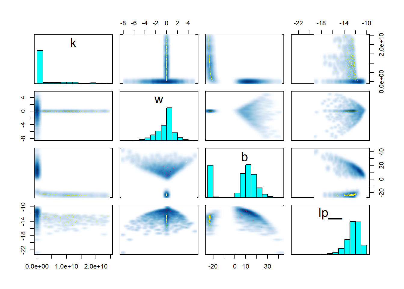
Clearly something substantial changed for the second model. But while there is a lot of stuff that looks fishy, it is hard to understand what exactly is going on. The clue is in looking at the interaction of \(w\), \(k\) and the log posterior (lp__) - you can play with the 3D plot below with your mouse. Note that ShinyStan provides similar 3D plots under Explore -> Trivariate.
samples <- rstan::extract(fit_sigmoid2_divergent)
open3d() %>% invisible()
rgl::plot3d(samples$w, samples$k, samples$lp__, xlab = "w", ylab = "k", zlab = "lp__")
The thing to notice here is that for \(w = 0\), there is a thin ridge in the posterior with almost maximal lp__ for a wide range of values for \(k\). This is because for \(w = 0\), the posterior ceases to depend on \(x\) and \(k\) becomes very closely tied to \(b\) - simultaneously almost any value of \(k\) that is admitted by the prior becomes feasible with suitable value of \(b\). The ridge is so thin, that the sampler almost completely misses it and it is barely visible in the plot. But for the true posterior, this ridge should contribute a non-trivial amount of mass. Once again, the sampler adapts its step size to the wide distribution for \(w \neq 0\) which leads to divergences and rejections when traversing the narrow ridge at \(w = 0\), bringing the problem to our attention.
What can you do about these kinds of problems? When you fit your model interactively, the best solution is to spot that your actual data are a special case and simplify your model. Special cases however become more of a worry when you need to automatically fit the model to a large number of datasets or refit it periodically as new data become available. The best solution I have found so far is to try fitting a simplified model first (here something like \(x \sim N(a,\sigma)\)). If the simplified model fits well and/or the full model diverges, the results of the simplified model are preferred. If you know of a better solution, please let me know - it is directly relevant to my work on models of gene regulation! The link also contains more discussion of the reparametrizations I use to make this kind of models converge.
Take home message: Worry about degenerate special cases of your model. A 3D trivariate plot of two parameters vs. the posterior, makes it really neatly visible when your posterior is not unimodal.
Neural network: When ordering is not enough
At this point it would make sense to mention mixture models, but as those are covered by the aforementioned case study, we’ll go straight ahead to the desperate wilderness of models too broken to fix. And neural networks are a prime attraction in this godforsaken land.
We don’t need to go fancy. Let’s have a feedforward neural net with two inputs, two hidden layers of two neurons each and a single output neuron.
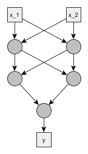
We will use the standard logistic sigmoid activation function and treat the problem as a binary classification. To make things simpler and because we saw that sigmoid may be non-dentifiable by itself, we ignore all the bias parameters, so the only parameters are the weights \(w\) of inputs \(x\) and the activation function becomes:
\[ \frac{1}{1+e^{-\sum w_i x_i}} \]
Below is the corresponding Stan model - optimized for readability, not brevity or generalizability. Since it seems there might be some symmetries, and we learned our lesson from mixture models, we’ll try at least to force the weights for the output neuron to be ordered.
stan_code_neural <- "


data {
  int N;
  matrix[N,2] x;
  int<lower=0, upper=1> y[N];
  real prior_width;
}

parameters {
  matrix[2,2] weights1;
  matrix[2,2] weights2;
  ordered[2] weights_out;
}

model {
  matrix[N,2] input1 = x * weights1;
  matrix[N,2] output1 = inv_logit(input1);

  matrix[N,2] input2 = output1 * weights2;
  matrix[N,2] output2 = inv_logit(input2);

  vector[N] input_out = output2 * weights_out;
  vector[N] output_out = inv_logit(input_out);
  y ~ bernoulli(output_out);

  to_vector(weights1) ~ normal(0, prior_width);
  to_vector(weights2) ~ normal(0, prior_width);
  weights_out ~ normal(0, prior_width);
}
"

model_neural <- stan_model(model_code = stan_code_neural)
In the spirit of the best traditions of the field of machine learning, we’ll try to teach XOR to the neural network. It does not go well. To make the pathologies better visible, we will use 8 chains instead of the usual 4.
set.seed(1324578)
sigma <- 0.1
N <- 200

x <- array(as.integer(rbernoulli(N * 2)), c(N,2))
y <- xor(x[,1], x[,2])

data_neural <- list(N = N, x = x, y = y, sigma = sigma, prior_width = 5)
fit_neural <- sampling(model_neural, data = data_neural, chains = 8)
## Warning: There were 178 divergent transitions after warmup. See
## https://mc-stan.org/misc/warnings.html#divergent-transitions-after-warmup
## to find out why this is a problem and how to eliminate them.## Warning: Examine the pairs() plot to diagnose sampling problems## Warning: The largest R-hat is 2.34, indicating chains have not mixed.
## Running the chains for more iterations may help. See
## https://mc-stan.org/misc/warnings.html#r-hat## Warning: Bulk Effective Samples Size (ESS) is too low, indicating posterior means and medians may be unreliable.
## Running the chains for more iterations may help. See
## https://mc-stan.org/misc/warnings.html#bulk-ess## Warning: Tail Effective Samples Size (ESS) is too low, indicating posterior variances and tail quantiles may be unreliable.
## Running the chains for more iterations may help. See
## https://mc-stan.org/misc/warnings.html#tail-essshow_param_diags <- function(fit) {
summary(fit)$summary[,c("n_eff","Rhat")]
}
show_param_diags(fit_neural)## n_eff Rhat
## weights1[1,1] 4.586133 2.842062
## weights1[1,2] 4.806146 2.472001
## weights1[2,1] 4.904083 2.345798
## weights1[2,2] 4.705657 2.597202
## weights2[1,1] 4.503922 3.078342
## weights2[1,2] 4.815908 2.502825
## weights2[2,1] 4.626493 2.776578
## weights2[2,2] 5.432725 1.999367
## weights_out[1] 4.433889 3.237023
## weights_out[2] 4.896132 2.350218
## lp__ 4.061244 8.279744We note the divergences, very low n_eff and large Rhat. Remember that n_eff (effective sample size) is a measure of how well the posterior was sampled and Rhat is close to one if the chains have converged to the same posterior. This time let’s start by inspecting some traceplots - I chose the ones I consider most interesting but in practice you would want to look at all of them (once again those are also available in ShinyStan):
fit_for_bayesplot <- as.array(fit_neural)
mcmc_trace(fit_for_bayesplot, pars = c("weights2[1,2]","weights1[2,2]"),
           facet_args = list(ncol = 1)) + scale_color_discrete()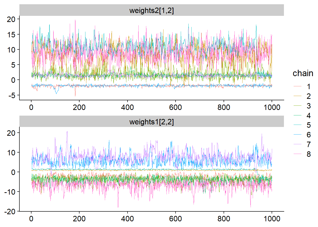
We clearly see that there are multiple modes and each chain is stuck in its mode and does not mix with others. The first trace plot shows that just investigating the marginal posterior for weights2[1,2] reveals 3 well separated modes. Looking at the traceplot for weights1[2,2] we see that there have to be even more modes as here, chain 2 (green-brown-ish?) clusters with chain 5 (blue), while in the first traceplot it clusters with chain 8 (pink).
Looking at the pairs plot provides some additional hints:
pairs(fit_neural, pars = c("weights2[1,2]","lp__"))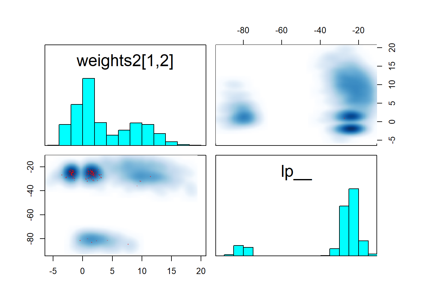
We see that at least the two “denser” modes are symmetric across zero and that they reach about the same maximum lp__ as the “diffuse” mode. This means that to identify the model we need have to somehow choose one of those modes, but there is clearly not a “best” (much higher lp__) mode.
My best guess is that the divergences arise when the sampler (unsuccesfully) tries to switch between individual modes and the geometry gets narrower in some parameters and wider in others, but this is just guesswork.
There is not really much that can be done to make such models work. The most obvious issues come from symmetries of the network structure, providing multiple modes when the neurons are relabelled, but the network is isomorphic. To some extent we could get rid of them by ordering one of the weights in each layer. However, ordering is just the start and further issues just keep on coming - see for example the forum thread on Bayesian neural networks for more details.
Take home message: Non overlaping traces without treedepth warnings indicate multimodality. If the modes have about the same lp__, some symmetry breaking constraints may help. If there is one mode with much larger lp__ than the others, it might make sense to favor this one by appropriate priors/reparametrization.
A hopelessly non-identified GP model
In the above example, there were multiple discrete and well separated modes. But there is still a way to move non-identifiability to the next level. We’ll start with a simple and harmless Gaussian process model with squared exponential covariance function, the model is:
\[ \begin{align} y_{est} &\sim GP(\rho,\tau) \\ y &\sim~ N(y_{est}(x), \sigma) \end{align} \]
Here, \(x \in (0,1)\) are the locations where the GP is observed. The corresponding Stan code is:
stan_code_gp <- "
data {
  int N;
  real x[N];
  vector[N] y;
  real<lower=0> gp_length;
  real<lower=0> gp_scale;
  real<lower=0> sigma;
}

transformed data {
  vector[N] mu = rep_vector(0, N);
}

parameters {
  vector[N] y_est_raw;
}

transformed parameters {
  vector[N] y_est;
  // Using the latent variable GP coding form Stan manual,
  // with the Cholesky decomposition
  {
    matrix[N, N] L_K;
    matrix[N, N] K = cov_exp_quad(x, gp_scale, gp_length);
    for (n in 1:N) {
      K[n, n] = K[n, n] + 1e-12; //Ensure positive definite
    }
    L_K = cholesky_decompose(K);
    y_est = L_K * y_est_raw;
  }
}

model {
  y ~ normal(y_est, sigma);
  y_est_raw ~ normal(0, 1);
}

"

model_gp <- stan_model(model_code = stan_code_gp)
We simulate some data and check that the model works well:
set.seed(25748422)
simulate_gp <- function(x) {
  N <- length(x)
  gp_length <- 0.3
  gp_scale <- 1
  sigma <- 0.1
  cov_m <- matrix(0, nrow <- N, ncol <- N)
  for(i in 1:N) {
    for(j in i:N) {
      cov_m[i,j] <- gp_scale ^ 2 * exp(-0.5 * (1 / gp_length ^ 2) * (x[i] - x[j])^2)
      cov_m[j,i] <- cov_m[i,j]
    }
  }
  chol_cov_m <- chol(cov_m)
  y <- chol_cov_m %*% rnorm(N, 0, 1)

  list(N = N, x = x, y = array(y, N), gp_length = gp_length, gp_scale = gp_scale, sigma = sigma)
}

data_gp <- simulate_gp(x = seq(0.01,0.99, length.out = 10))
fit_gp <- sampling(model_gp, data = data_gp)
show_param_diags(fit_gp) %>% head()
## n_eff Rhat
## y_est_raw[1] 3159.529 1.000177
## y_est_raw[2] 2315.263 1.000567
## y_est_raw[3] 1975.222 1.000598
## y_est_raw[4] 1860.736 1.001232
## y_est_raw[5] 2289.527 1.001320
## y_est_raw[6] 2555.396 1.001130We note the good diagnostics and also look at the posterior draws versus the observed values.
samples_to_show <- sample(1:4000, 50)
fit_gp %>%
  tidybayes::spread_draws(y_est[x_index]) %>%
  inner_join(data.frame(x_index = 1:data_gp$N, x = data_gp$x), by = c("x_index" = "x_index")) %>%
  mutate(sample_id = (.chain - 1) * 1000 + .iteration ) %>%
  filter(sample_id %in% samples_to_show) %>%
  ggplot(aes(x = x, y = y_est, group = sample_id, color = as.factor(.chain))) + geom_line(alpha = 0.3) +
  geom_point(data = data.frame(x = data_gp$x, y = data_gp$y), aes(x = x, y = y), inherit.aes = FALSE)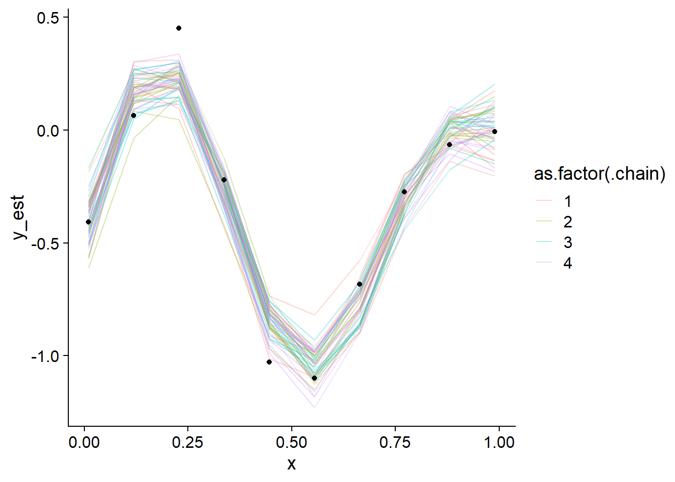
And now a magic trick that turns this well-behaved model into a mess: we’ll treat \(x\), the locations where the GP is observed as unknown. Since \(x \in (0,1)\), we can specify a Beta prior for the locations with varying precision. The modified Stan code follows.
stan_code_gp_mess <- "
data {
  int N;
  vector[N] y;
  real<lower=0> gp_length;
  real<lower=0> gp_scale;
  real<lower=0> sigma;
  vector<lower=0, upper=1>[N] x_prior_mean;
  real<lower=0> x_prior_tau;
}

transformed data {
  vector[N] mu = rep_vector(0, N);
}

parameters {
  real<lower=0, upper = 1> x[N];
  vector[N] y_est_raw;
}

transformed parameters {
  vector[N] y_est;
  // Using the latent variable GP coding form Stan manual,
  // with the Cholesky decomposition
  {
    matrix[N, N] L_K;
    matrix[N, N] K = cov_exp_quad(x, gp_scale, gp_length);
    for (n in 1:N) {
      K[n, n] = K[n, n] + 1e-12; //Ensure positive definite
    }
    L_K = cholesky_decompose(K);
    y_est = L_K * y_est_raw;
  }
}

model {
  y ~ normal(y_est, sigma);
  y_est_raw ~ normal(0, 1);
  x ~ beta(x_prior_mean * x_prior_tau,  (1 - x_prior_mean) * x_prior_tau);
}

"

model_gp_mess <- stan_model(model_code = stan_code_gp_mess)
Let’s start with noninformative uniform prior on \(x\).
set.seed(42148744)

data_gp_mess_uniform <- data_gp
#This puts uniform prior on all x
data_gp_mess_uniform$x_prior_mean = rep(0.5, data_gp$N)
data_gp_mess_uniform$x_prior_tau = 2

fit_gp_mess <- sampling(model_gp_mess, data = data_gp_mess_uniform)
## Warning: There were 565 divergent transitions after warmup. See
## https://mc-stan.org/misc/warnings.html#divergent-transitions-after-warmup
## to find out why this is a problem and how to eliminate them.## Warning: There were 2185 transitions after warmup that exceeded the maximum treedepth. Increase max_treedepth above 10. See
## https://mc-stan.org/misc/warnings.html#maximum-treedepth-exceeded## Warning: Examine the pairs() plot to diagnose sampling problems## Warning: The largest R-hat is 2.51, indicating chains have not mixed.
## Running the chains for more iterations may help. See
## https://mc-stan.org/misc/warnings.html#r-hat## Warning: Bulk Effective Samples Size (ESS) is too low, indicating posterior means and medians may be unreliable.
## Running the chains for more iterations may help. See
## https://mc-stan.org/misc/warnings.html#bulk-ess## Warning: Tail Effective Samples Size (ESS) is too low, indicating posterior variances and tail quantiles may be unreliable.
## Running the chains for more iterations may help. See
## https://mc-stan.org/misc/warnings.html#tail-essshow_param_diags(fit_gp_mess) %>% head()## n_eff Rhat
## x[1] 2.111522 4.678524
## x[2] 2.081677 5.845164
## x[3] 2.064901 6.388092
## x[4] 2.100400 5.438441
## x[5] 2.046444 6.949529
## x[6] 11.013634 1.391479We can note that we got both divergences and max treedepth, meaning that the step size is sometimes too large and sometimes too small, also both n_eff and Rhat are atrocious. Let’s inspect some traces:
fit_for_bayesplot <- as.array(fit_gp_mess)
mcmc_trace(fit_for_bayesplot, pars = c("x[1]","y_est[1]", "lp__"), facet_args = list(ncol = 1)) + scale_color_discrete()
## Scale for 'colour' is already present. Adding another scale for 'colour',
## which will replace the existing scale.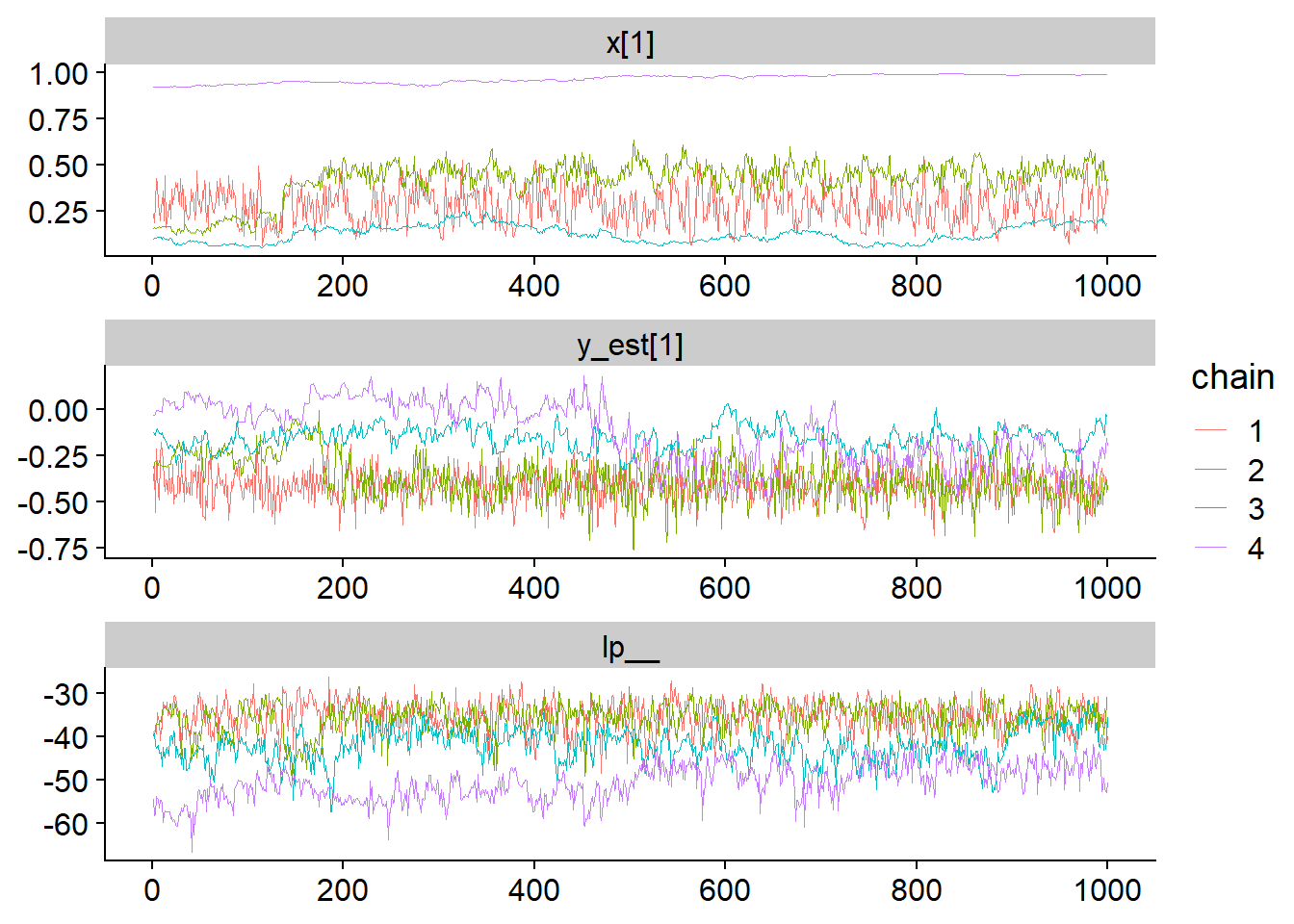
In contrast to the neural net example, here the chains do not stick to a single mode, instead, they slowly wander across a wide range of values. Further, we see that the log posterior more or less overlaps across the explored parts of the parameter space. How does that look like when we plot the posterior?
plot_gp_mess <- function(fit_gp_mess) {
  samples_to_show <- sample(1:4000, 50)
  fit_gp_mess %>%
    tidybayes::spread_draws(y_est[x_index], x[x_index]) %>%
    mutate(sample_id = (.chain - 1) * 1000 + .iteration ) %>%
    filter(sample_id %in% samples_to_show) %>%
    ggplot(aes(x = x, y = y_est, group = sample_id, color = as.factor(.chain))) + geom_line(alpha = 0.3) +
    geom_point(data = data.frame(x = data_gp$x, y = data_gp$y), aes(x = x, y = y), inherit.aes = FALSE)
}

plot_gp_mess(fit_gp_mess)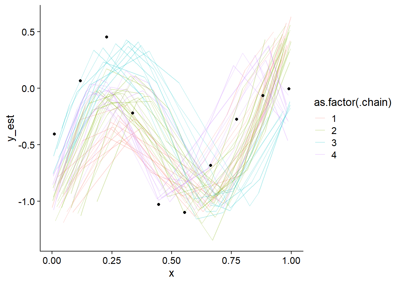
Not even close! We also see that the chains actually do sample different regions of the whole posterior, despite overlapping in marginal posteriors. Lets also take a look at some pairs plots:
pairs(fit_gp_mess, pars = c("x[1]","y_est[1]", "lp__"))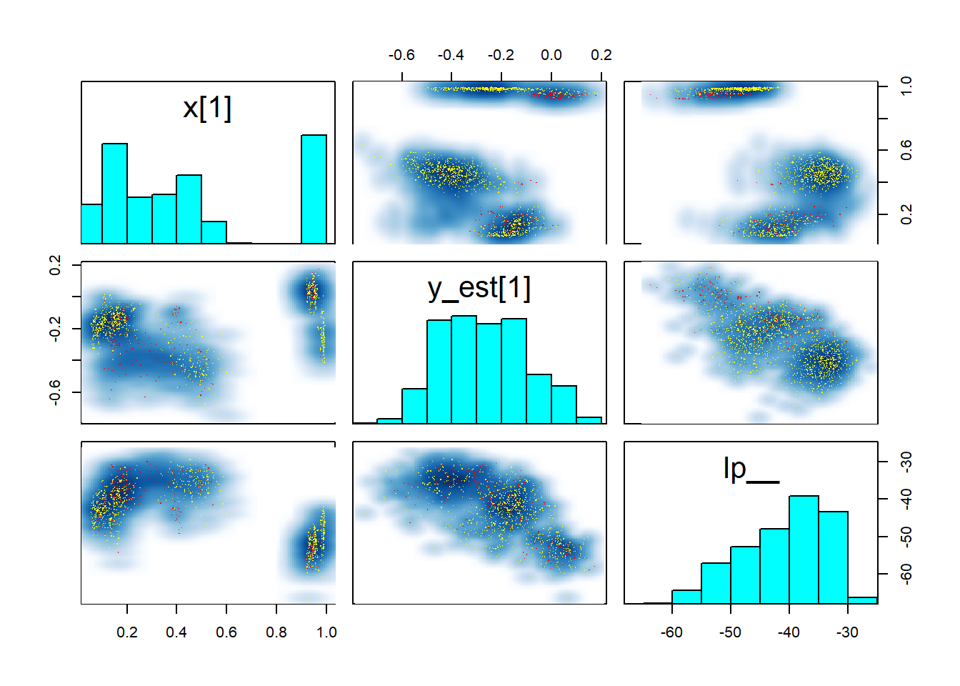
Those pairs are not of much help, except that they once again show that there is no clean separation in log posterior (lp__) between the individual modes. Taken together this indicates that the posterior likely has many modes connected by thin, possibly curved ridges with only slightly smaller lp__. This is not surprising, since ordering of \(x\) is only weakly constrained by the GP variance (when \(x\) is close together, \(y\) should be as well). In fact, we would expect the number of modes to be of order \(N!\) (factorial of \(N\)).
A nice diagnostic trick is to set informative priors on \(x\), centered on the true values. The width of the prior required to make the model identified tells us something about the severity of the issues. This is where the Beta prior, in particular it’s parametrization via mean and precision (\(\tau\)) comes in handy. So, lets see if \(\tau = 1000\), e.g. the amount of information contained in 1000 coin flips is enough. Note that we also have to init the chains around the true values, otherwise the sharp prior introduces sampling problems.
set.seed(741284)
data_gp_mess_informed <- data_gp
data_gp_mess_informed$x_prior_mean = data_gp$x
data_gp_mess_informed$x_prior_tau = 1000

informed_init <- function(){
  list(x = data_gp$x)
}

fit_gp_mess_informed <- sampling(model_gp_mess, data = data_gp_mess_informed, init = informed_init)
show_param_diags(fit_gp_mess_informed) %>% head()
## n_eff Rhat
## x[1] 7807.223 0.9996608
## x[2] 6203.740 1.0000260
## x[3] 7690.874 0.9993963
## x[4] 6966.835 0.9993572
## x[5] 7530.549 0.9993165
## x[6] 7651.445 0.9992267plot_gp_mess(fit_gp_mess_informed)## Warning: 'tidybayes::spread_samples' is deprecated.
## Use 'spread_draws' instead.
## See help("Deprecated") and help("tidybayes-deprecated").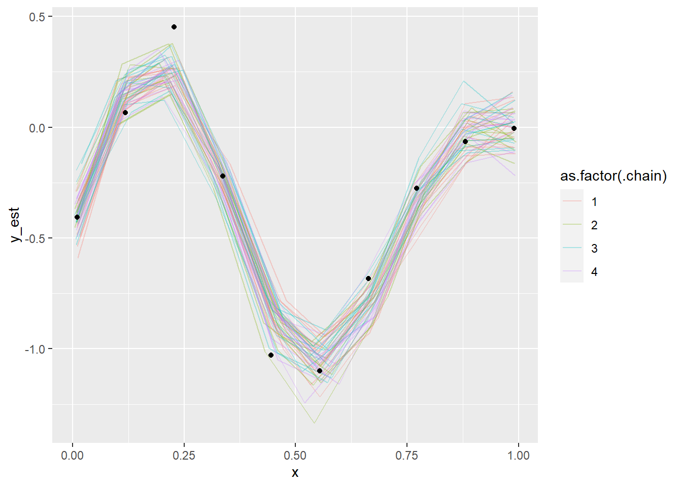
And it indeed is enough, the diagnostics look good, the posterior looks good, everything’s peachy. But we needed a very narrow prior. And we could not get away with much less information, consider setting \(\tau = 500\) (still a very narrow prior):
set.seed(32148422)
data_gp_mess_less_informed <- data_gp
data_gp_mess_less_informed$x_prior_mean = data_gp$x
data_gp_mess_less_informed$x_prior_tau = 500

fit_gp_mess_less_informed <- sampling(model_gp_mess, data = data_gp_mess_less_informed, init = informed_init)
## Warning: There were 3 divergent transitions after warmup. See
## https://mc-stan.org/misc/warnings.html#divergent-transitions-after-warmup
## to find out why this is a problem and how to eliminate them.## Warning: Examine the pairs() plot to diagnose sampling problemsshow_param_diags(fit_gp_mess_less_informed) %>% head()## n_eff Rhat
## x[1] 6299.314 0.9995523
## x[2] 6007.538 0.9992767
## x[3] 6495.730 0.9996561
## x[4] 6313.321 1.0002979
## x[5] 6340.341 1.0005830
## x[6] 6331.998 0.9991734plot_gp_mess(fit_gp_mess_less_informed)## Warning: 'tidybayes::spread_samples' is deprecated.
## Use 'spread_draws' instead.
## See help("Deprecated") and help("tidybayes-deprecated").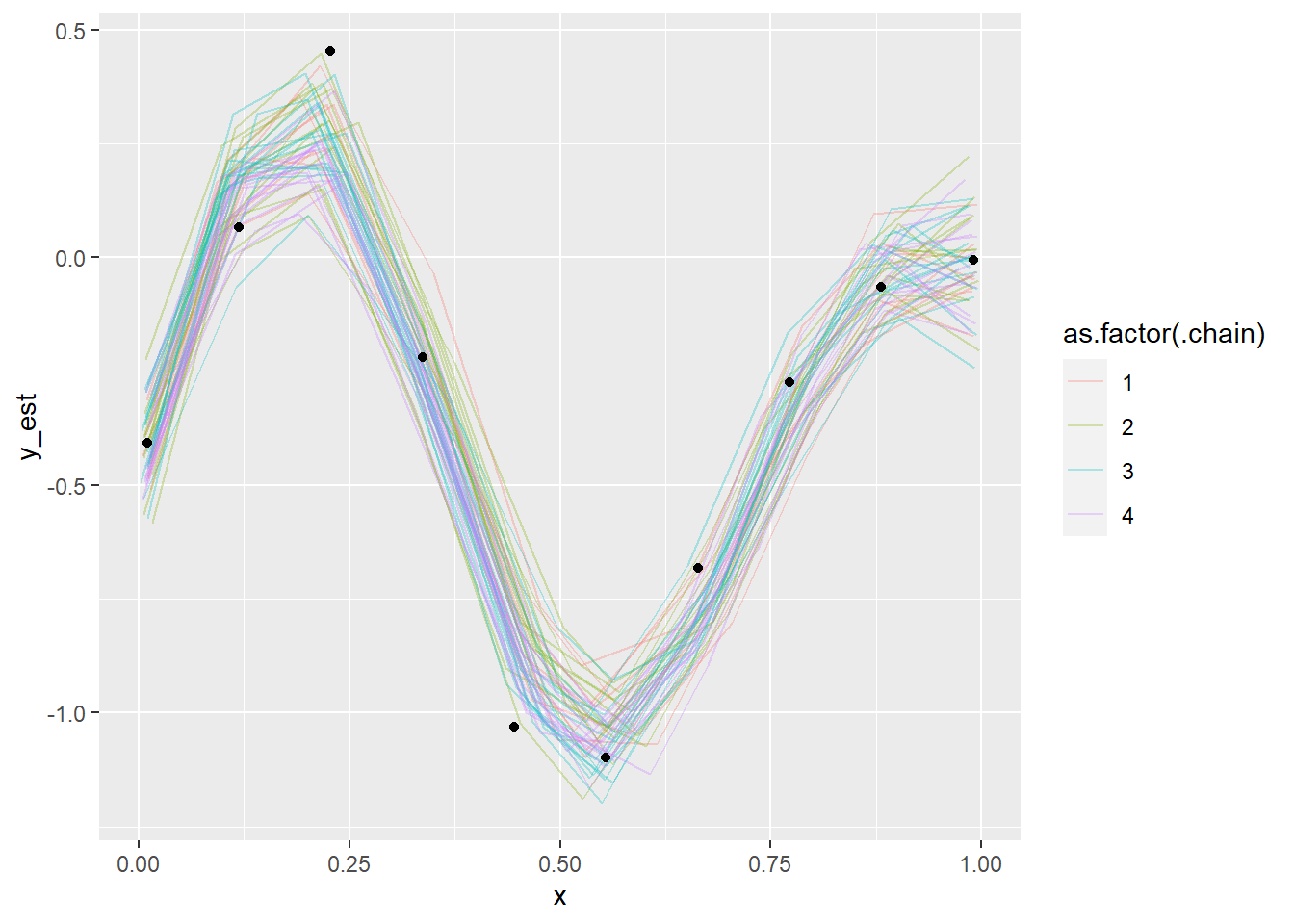
Even though the posterior looks more or less OK, we see that the chains have not mixed well (notably, chain 2 forms a slightly separate cluster) as also indicated by some of the diagnostics. So we can conclude that the model is screwed as it is not identified, unless we already now the values of \(x\) quite precisely.
Take home message: Chains wandering slowly across large areas of posterior but with roughly the same lp__ is a very bad sign. Putting narrow priors centered on true parameters is a neat trick to understand your model better.
Conclusion
That’s it - if you’ve made it to the bottom of this looooong post, you are great and thanks very much! I really hope that it will help you interpret your own models and help determine how to fix them or when to abandon a hopeless situation and get back to the drawing board. I also hope I have convinced you that identifiability depends not only on the model but also on the actual observed dataset.
Best of luck with modelling!
Computing environment
sessionInfo()## R version 4.1.0 (2021-05-18)
## Platform: x86_64-w64-mingw32/x64 (64-bit)
## Running under: Windows 10 x64 (build 19044)
##
## Matrix products: default
##
## locale:
## [1] LC_COLLATE=Czech_Czechia.1250 LC_CTYPE=Czech_Czechia.1250
## [3] LC_MONETARY=Czech_Czechia.1250 LC_NUMERIC=C
## [5] LC_TIME=Czech_Czechia.1250
##
## attached base packages:
## [1] stats graphics grDevices utils datasets methods base
##
## other attached packages:
## [1] rgl_0.108.3 here_1.0.1 knitr_1.38 tidybayes_3.0.1
## [5] bayesplot_1.8.1 rstan_2.26.6 StanHeaders_2.26.6 forcats_0.5.1
## [9] stringr_1.4.0 dplyr_1.0.7 purrr_0.3.4 readr_2.1.0
## [13] tidyr_1.1.4 tibble_3.1.6 ggplot2_3.3.5 tidyverse_1.3.1
##
## loaded via a namespace (and not attached):
## [1] colorspace_2.0-2 ellipsis_0.3.2 ggridges_0.5.3
## [4] rprojroot_2.0.2 fs_1.5.2 rstudioapi_0.13
## [7] farver_2.1.0 svUnit_1.0.6 fansi_0.5.0
## [10] lubridate_1.8.0 xml2_1.3.2 codetools_0.2-18
## [13] extrafont_0.17 cachem_1.0.6 jsonlite_1.7.2
## [16] broom_0.8.0 Rttf2pt1_1.3.9 dbplyr_2.1.1
## [19] ggdist_3.0.0 compiler_4.1.0 httr_1.4.2
## [22] backports_1.3.0 assertthat_0.2.1 fastmap_1.1.0
## [25] cli_3.2.0 htmltools_0.5.2 prettyunits_1.1.1
## [28] tools_4.1.0 coda_0.19-4 gtable_0.3.0
## [31] glue_1.6.2 reshape2_1.4.4 posterior_1.1.0.9000
## [34] V8_3.6.0 Rcpp_1.0.7 cellranger_1.1.0
## [37] jquerylib_0.1.4 pkgdown_2.0.1 vctrs_0.3.8
## [40] blogdown_1.6 extrafontdb_1.0 tensorA_0.36.2
## [43] xfun_0.30 ps_1.6.0 rvest_1.0.2
## [46] lifecycle_1.0.1 scales_1.1.1 hms_1.1.1
## [49] parallel_4.1.0 inline_0.3.19 yaml_2.2.1
## [52] curl_4.3.2 memoise_2.0.0 gridExtra_2.3
## [55] loo_2.4.1 sass_0.4.0 stringi_1.7.5
## [58] highr_0.9 checkmate_2.0.0 pkgbuild_1.2.0
## [61] rlang_0.4.12 pkgconfig_2.0.3 matrixStats_0.61.0
## [64] distributional_0.2.2 evaluate_0.15 lattice_0.20-44
## [67] htmlwidgets_1.5.4 labeling_0.4.2 cowplot_1.1.1
## [70] processx_3.5.2 tidyselect_1.1.1 plyr_1.8.6
## [73] magrittr_2.0.1 bookdown_0.24 R6_2.5.1
## [76] generics_0.1.1 DBI_1.1.1 pillar_1.6.4
## [79] haven_2.4.3 withr_2.4.2 abind_1.4-5
## [82] modelr_0.1.8 crayon_1.4.2 arrayhelpers_1.1-0
## [85] KernSmooth_2.23-20 utf8_1.2.2 tzdb_0.2.0
## [88] rmarkdown_2.11 grid_4.1.0 readxl_1.3.1
## [91] callr_3.7.0 reprex_2.0.1 digest_0.6.28
## [94] RcppParallel_5.1.4 stats4_4.1.0 munsell_0.5.0
## [97] bslib_0.3.1