I am not a staunch advocate of Bayesian methods — I can totally see how for some questions a frequentist approach may provide more satisfactory answers. In this post, we’ll explore how for a simple scenario (negative binomial regression with small sample size), standard frequentist methods fail at being frequentist while standard Bayesian methods provide good frequentist guarantees.
A bit of theory
First, lets make sure we all agree what we are talking about. Those comfortable with Bayesian and frequentist calibration may safely skip to the next section.
For simplicity, we will focus on uncertainty intervals for a continuous parameter. A frequentist will construct a confidence interval (CI) which should satisfy the following requirement:
For any fixed parameter value, \(x\%\) CI contains the true value at least \(x\%\) of the time.
In other words, we are aiming to control worst case behaviour. We also note that CIs do not require exact coverage, but put a lower bound on coverage — this is primarily because in many settings a CI with exact coverage may not exist (i.e. to obtain sufficient coverage in the worst case, one must settle for larger than nominal coverage elsewhere). CIs are closely related to frequentist tests as any hypothesis outside of \(1 - \alpha\) CI can be rejected at \(\alpha\) level.
A Bayesian will typically compute a credible interval (CrI), which has a slightly different property:
Averaged over the prior, \(x\%\) CrI contains the true value exactly \(x\%\) of the time.
So instead of worst case we are looking at the average case. We explicitly accept that specific parameter values may lead to low coverage as long as other parameter values lead to higher coverage. On the other hand, we are often able to compute exact1 credible intervals achieveng precisely the desired coverage.
To highlight the difference, we will use a simple “coin flipping” scenario:
\[ Y \sim \text{Binomial}(20, \theta) \]
And assume a Bayesian would use a uniform prior:
\[ \theta \sim \text{Uniform}(0,1) \]
In this setting, we can do reliable frequentist inference with the Clopper-Pearson interval or obtain a Bayesian posterior via the Beta distribution \(\pi(\theta | Y = y) = \text{Beta}(y + 1, 20 - y + 1)\).
Let’s look on the coverage of the Clopper-Pearson interval as well as a credible interval, specifically the 95% highest posterior density interval2 for all possible values of \(\theta\):
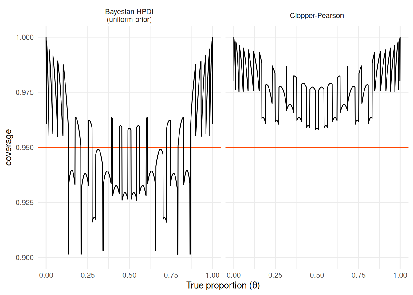
We see that the Clopper-Pearson interval is conservative: it always achieves at least 95% coverage (sometimes much larger), regardless of the true proportion (\(\theta\)). OTOH, the Bayesian HPDI has higher coverage for some values and lower for others — in fact the area above the red horizontal line (nominal calibration) is exactly equal to the area under and thus we have exactly 95% coverage when averaged over uniform prior. The Clopper-Pearson intervals would naturally be a bit wider than the Bayesian HPDI. We also see that discrete data make the plot look pretty wild.
The curious case of the negative binomial
To show a situation where standard frequentist intervals don’t perform so well, we are going to fit a negative binomial regression model, with 2 groups. Technically:
\[ y_i \sim NB(\mu_i, \phi) \\ \log\mu_i = \alpha + \beta \times \text{group}_i \]
where \(\text{group}_i\) is a binary indicator of group membership.
For the frequentist side, we will be using MASS package:
MASS::glm.nb(y ~ group, data = data)as well as the gamlss package:
gamlss::gamlss(y ~ group, family = "NBI")and the glmmTMB package:
glmmTMB::glmmTMB(y ~ group, family = glmmTMB::nbinom2, data = data)on the Bayesian side, we’ll use the brms package with flat priors:
brms::brm(y ~ group, data = data, family = "negbinomial",
  prior = brms::prior("", class = "Intercept"))
(the results don’t change much if we keep the default prior).
Note that frequentist coverage needs to hold for any true parameter value, so proving a frequentist method works is hard, but finding even a single set of parameters where the coverage does not hold invalidates the method (strictly speaking).
We will focus on a small-sample scenario with 4 observations in each group. As a check, we will also include large-sample scenario with 100 observations in each group.
To cover a range of somewhat realistic scenarios, we will use a single value of \(\alpha = \log(100)\), and iterate over 10 values of \(\beta\) equally spaced between \(0\) and \(2\) and \(\phi \in \{0.5, 1, 2.5, 10\}\).
Typically \(\beta\) is the parameter of interest, so we will examine its coverage and we won’t care about the coverage for \(\alpha\) and \(\phi\) as that’s tangential (and packages rarely optimize for those parameters).
Here is our simulation code (note that we make sure to always use exactly the same dataset with all packages):
sim_nb_coverage_single <- function(N_per_group, mu, b, phi, sim_id, base_brm) {
  group <- c(rep(0, N_per_group), rep(1, N_per_group))

  y <- rnbinom(2 * N_per_group, mu = exp(mu + b * group), size = phi)
  data <- data.frame(y, group)

  cf_glm.nb <- suppressMessages(confint(MASS::glm.nb(y ~ group, data = data))[2, ])

  cf_gamlss <- tryCatch({
    fit_gamlss <- gamlss::gamlss(y ~ group, family = "NBI", data = data)
    confint(fit_gamlss)[2, ]
  }, error = function(e) {
    return(c(NA, NA))
  })


  cf_glmmTMB <- tryCatch({
    m <- glmmTMB::glmmTMB(y ~ group, family = glmmTMB::nbinom2, data = data)
    confint(m,
            method = "profile",
            parm = "group",
            estimate = FALSE)
  }, error = function(e) {
    return(c(NA, NA))
  })


  # Rarely we get problematic init which results in fitted phi -> infty and bad BFMI
  # refitting fixes that (more informative prior on phi also would)
  for (i in 1:5) {
    fit_brm <- update(
      base_brm,
      newdata = data,
      cores = 1,
      chains = 2,
      future = FALSE,
      refresh = 0
    )

    if (all(!is.na(rstan::get_bfmi(fit_brm$fit)))) {
      break
    }
  }

  bfmi_problem <- any(is.na(rstan::get_bfmi(fit_brm$fit)))
  cf_brm <- brms::fixef(fit_brm)["group", c(3, 4)]

  data.frame(
    method = c("glm.nb", "glmmTMB", "gamlss", "brms"),
    sim_id,
    mu = mu,
    b = b,
    phi = phi,
    N_per_group = N_per_group,
    ci_low = unname(c(
      cf_glm.nb[1], cf_glmmTMB[1], cf_gamlss[1], cf_brm[1]
    )),
    ci_high = unname(c(
      cf_glm.nb[2], cf_glmmTMB[2], cf_gamlss[2], cf_brm[2]
    )),
    bfmi_problem = c(FALSE, FALSE, FALSE, bfmi_problem)
  )
}
Now we just run it (+cache results)
coverage_cache_file <- file.path(cache_dir, "nb_coverage.rds")
if(!file.exists(coverage_cache_file)) {


  # Construct base brms object to update
  mu_0 <- log(100)
  group_eff <- log(1.5)
  true_phi <- 2.5
  group <- c(rep(0, 4), rep(1, 4))
  y <- rnbinom(8, mu = exp(mu_0 + group_eff * group), size = true_phi)
  prior <- c(brms::prior("", class = "Intercept"))
  base_brm <- brms::brm(
    y ~ group,
    data = data.frame(y, group),
    family = "negbinomial",
    prior = prior,
    backend = "cmdstanr"
  )


  scenarios <- tidyr::crossing(
    N_per_group = c(4, 100),
    mu = log(100),
    b = seq(0, 2, length.out = 10),
    phi = c(0.5, 1, 2.5, 10),
    sim_id = 1:1000
  )


  nb_coverage_df <- furrr::future_pmap_dfr(
    scenarios,
    \(...) sim_nb_coverage_single(..., base_brm = base_brm),
    .options = furrr::furrr_options(seed = TRUE, chunk_size = 40)
  )

  saveRDS(nb_coverage_df, file = coverage_cache_file)
} else {
  nb_coverage_df <- readRDS(coverage_cache_file)
}
And we plot the results for \(4\) observations per group — showing the coverage + dark gray band is the the remaining uncertainty about the coverage (via the Clopper-Pearson interval):
coverage_plot <- function(coverage_df) {
  coverage_df |>
    filter(!is.na(ci_low), !is.na(ci_high)) |>
    mutate(
      covered = b >= ci_low & b <= ci_high,
      `φ` = phi,
      method = factor(method, levels = c("brms", "glmmTMB", "gamlss", "glm.nb"))
    ) |>
    group_by(method, b, phi, `φ`) |>
    summarise(
      coverage = mean(covered),
      n_covered = sum(covered),
      coverage_low = qbeta(0.025, n_covered, n() - n_covered + 1),
      coverage_high = qbeta(0.975, n_covered + 1 , n() - n_covered),
      .groups = "drop"
    ) |>
    ggplot()  + aes(
      x = b,
      ymin = coverage_low,
      y = coverage,
      ymax = coverage_high
    ) +
    geom_hline(color = "orangered", yintercept = 0.95) +
    geom_ribbon(fill = "#888", alpha = 0.3) +
    geom_line() + facet_grid(`φ` ~ method, labeller = "label_both") +
    scale_y_continuous("Coverage", labels = scales::percent) +
    scale_x_continuous("True β") + theme(strip.text.y = element_text(size = 10))
}

nb_coverage_df |> filter(N_per_group == 4) |> coverage_plot()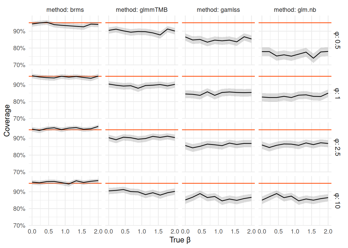
We see that glm.nb performs pretty badly with coverage of the 95% CI fluctuating between ~75% and ~90%.
The gamlss intervals are only slightly better and glmmTMB is yet better but still staying close to 90% coverage for all settings.
In other words, all of the frequentist intervals are too narrow.
On the other hand brms provides very close to nominal frequentist coverage for all tested parameter values,
despite not technically claiming that guarantee.
So what did happen to the frequentist packages?
Frequentist computation is HARD
There is a dirty secret behind most commonly used frequentist methods — except for a few special cases (e.g., standard linear regression, the aforementioned Clopper-Pearson interval) they are only only approximations that are justified by their behaviour in the large-data limit, but which have no strict guarantees in small datasets. Actual honest small-sample-guaranteed frequentist computation is hard for non-trivial models and often requires solutions specific to a single class of models.
The two most-commonly found approximations are:
- Normal (also sometimes called “Wald”) - this relies on the normal approximation to the likelihood around the maximum-likelihood estimate, usually
also accounting for additional uncertainty due to a scale parameter being estimated by using a Student’s t-distribution with appropriate number of degrees of freedom. In our example,
gamlssderives CIs via the t distribution. - Profile likelihood CIs which are derived from the \(\chi^2\) approximation in the likelihood-ratio test (i.e. any value that wouldn’t be rejected by a likelihood ratio test at \(5\%\) is included in the \(95\%\) CI).
In our example both
glm.nbandglmmTMBcompute profile confidence intervals (glmmTMBcomputes Wald intervals by default, but we have setmethod = "profile"to get profile intervals asgamlssalready gave us Wald intervals).
It is generally agreed that profile confidence intervals typically have better performance in small samples, i.e. they approach the asymptotic regime faster than normal/Wald intervals.
The reason why glm.nb performs worse than gamlss and glmmTMB is that glm.nb is a wrapper around glm
which for technical reasons3 treats \(\phi\) as constant instead of optimizing it in the profile computation (as glmmTMB does), i.e.
any uncertainty in \(\phi\) is ignored when computing the CIs in glm.nb.
gamlss takes into account the uncertainty in \(\phi\) but uses a Wald interval, which (as expected) performs worse than the profile likelihood used in glmmTMB.
Since the packages included exhaust the common, general approaches to compute CIs, there is not much hope to get better coverage with another frequentist package, unless it implements some specialized method tailored specifically to negative binomial models.
On the contrary, brms uses MCMC and allows for “exact” (Bayesian) computation
regardless of sample size. It turns out that in this example, exact Bayesian answer is
much closer to a correct frequentist answer than approximate frequentist approaches.
Large data limit
As a check we show that as we increase the sample size to 100 per group, we see all packages to converge on nominal coverage (as in large sample limit all of the approaches are equivalent).
nb_coverage_df |> filter(N_per_group == 100) |> coverage_plot()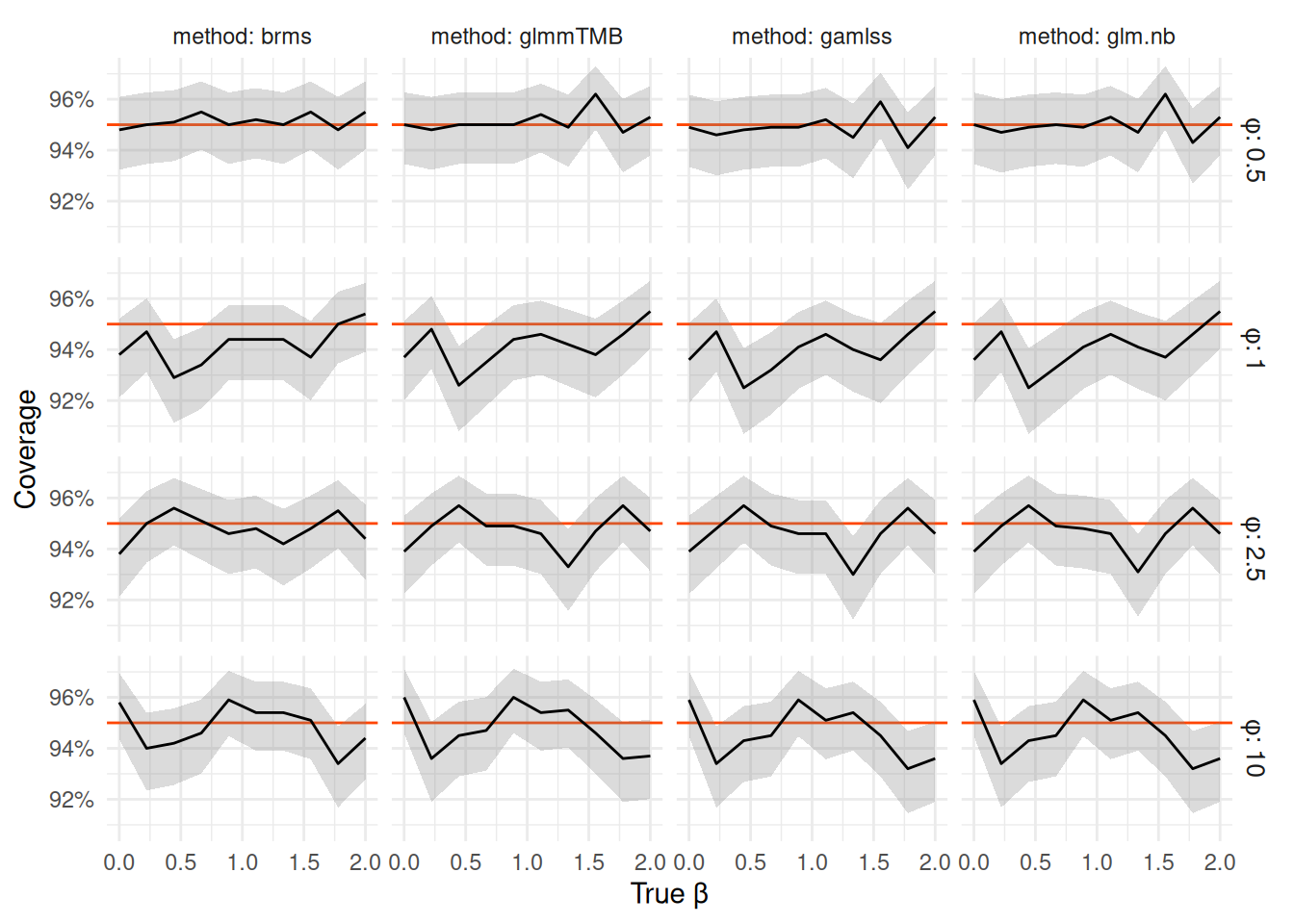
Note that the scale of the vertical axis has shrunk substantially and all the remaining coverages are within 92% - 96%.
In fact we can see that the
95% CI bounds for all methods are basically identical when we have 100 observations per group — in the table below we focus on
the distance between median of the lower/upper bound of all methods. The only slight difference is to brms where we hit the limits
of precision of the MCMC chains we ran, but except a few outliers (due to bad initialization, which could be resolved by even mild priors or just rerunning the chain) the bounds are within 0.1 of the other methods.
ci_match_summary <- function(coverage_df) {
  coverage_df |>
    group_by(sim_id, N_per_group, mu, b, phi) |>
    mutate(low = ci_low - median(ci_low),
           high = ci_high - median(ci_high)) |>
    pivot_longer(all_of(c("low", "high")), names_to = "bound", values_to = "value") |>
    group_by(method, bound) |>
    summarise(
      `Within 0.01` = sum(abs(value) < 0.01),
      `Outside 0.01` = sum(abs(value) >= 0.01),
      `Outside 0.1` = sum(abs(value) >= 0.1),
      .groups = "drop"
    )
}
nb_coverage_df |> filter(N_per_group == 100) |> ci_match_summary() |> knitr::kable()| method | bound | Within 0.01 | Outside 0.01 | Outside 0.1 |
|---|---|---|---|---|
| brms | high | 31411 | 8589 | 7 |
| brms | low | 31519 | 8481 | 7 |
| gamlss | high | 40000 | 0 | 0 |
| gamlss | low | 40000 | 0 | 0 |
| glm.nb | high | 40000 | 0 | 0 |
| glm.nb | low | 40000 | 0 | 0 |
| glmmTMB | high | 40000 | 0 | 0 |
| glmmTMB | low | 40000 | 0 | 0 |
Conclusions
The aim of this demonstration is an existential proof: there are practically relevant cases where fitting a Bayesian model with flat (or very wide) priors gives you better frequentist performance than common frequentist approaches.
I stumbled on this pretty randomly and I am not sure how common such situations are, but if anybody insists that frequentist tools are for some reason inherently superior to Bayesian, remember: most commonly used frequentist methods are approximations without strong small-sample guarantees. In such settings, even a staunch frequentist may be better served by Bayesian computation.
or precise enough, with MCMC↩︎
In many cases the central CrI will work well, but here it has unnecessary problems as even when we have all success or all failures, the central posterior interval does not include 0 or 1, but the highest posterior density interval does.↩︎
Because it delegates most of its work to
glmwhich requires an exponential family distribution. Neg. binomial with fixed \(\phi\) is exponential family but with \(\phi\) unknown it is not.glm.nbiteratively letsglmoptimize all paramters except \(\phi\) and then optimized \(\phi\) and then refits viaglmuntil convergence. But all methods on the fit (confint,predict, …) are delegated toglmwhich then keeps \(\phi\) at the ML estimate.↩︎