I recently needed to find the distribution of sum of non-identical but independent negative binomial (NB) random variables. Although for some special cases the sum is itself NB, analytical solution is not feasible in the general case. However it turns out there is a very handy tool called “Saddlepoint approximation” that is useful whenever you need densities of sums of arbitrary random variables. In this post I use the sum of NBs as a case study on how to derive your own approximations for basically any sum of independent random variables, show some tricks needed to get the approximation working in Stan and evaluate it against simpler approximations. To give credit where credit is due, I was introduced to the saddlepoint method via Cross Validated answer on sum of Gamma variables.
Spoiler: it turns out the saddlepoint approximation is not that great for actual inference (at least for the cases I tested), but it is still a cool piece of math and I spent too much researching it to not show you this whole post.
The Approximation - Big Picture
The saddlepoint approximation uses the cumulant-generating function (CGF) of a distribution to compute an approximate density at a given point. The neat part about CGFs is that the CGF of the sum of several variables is the sum of the individual CGFs! And CGFs are easy to come by, because the CGF is just the log of the moment-generating function and Wikipedia helpfully lists moment-generating functions for almost all distributions. Figuring out the CGF of almost any sum variable (including variables from different families) is thus relatively straightforward. The CGF can also easily be derived for general linear combinations of random variables.
The actual method for approximating density \(f\) at point \(x\), given the cumulant-generating function \(K\), and its first and second derivatives (\(K^\prime,K^{\prime\prime}\)) is as follows:
- find the saddlepoint \(s_x\) by solving:
\[ K^\prime(s_x) = x \]
Generally, there is no closed-form solution for \(s_x\), but since \(K(x)\) is always convex, \(K^\prime\) is always increasing, making it a nice target for numerical solutions. Still, since a different solution is needed for each \(x\), finding \(s_x\) tends to be a computational bottleneck.
- Once we have \(s_x\), we can approximate
\[ f(x) \simeq \frac1{\sqrt{2\pi K''(s_x)}} \exp(K(s_x) - x s_x) \]
The nice thing about the saddlepoint approximation is that it can easily produce approximations for both discrete and continous densities, and doesn’t constrain the approximation to be normal (unlike Laplace approximation). One thing to note is that the saddlepoint approximation in the form above does not necessarily integrate to 1, so a renormalization might be needed if you are interested in the actual density. But to use in Stan, unnormalized density is all that’s needed.
Saddlepoint for Sum of NBs
The moment-generating function of NB distribution parametrized by number of failures \(r\) and probability of success \(p\) is:
\[ M(t) = \left( \frac{1 - p}{1 - p e^t} \right)^r \]
So, taking the log and summing over \(n\) independent NB variables, the cumulant of sum of NB is:
\[ K(t) = \sum_{i=1}^{n} r_i \left[ \log(1-p_i) - \log(1 - p_i e^t) \right] \]
We now transform to the more useful parametrization of NB via mean \(\mu\) and precision \(\phi\) (i.e. \(Var(X) = \mu + \frac{\mu^2}{\phi}\)), where we have:
\[ r_i = \phi_i \\ p_i = \frac{\mu_i}{\phi_i + \mu_i} \\ K(t) = \sum_{i=1}^{n} \phi_i \left[ \log \frac{\phi_i}{\phi_i + \mu_i} - \log \left(1 - \frac{\mu_i e^t}{\phi_i + \mu_i} \right) \right] = \\ =\sum_{i=1}^{n} \phi_i \left[ \log(\phi_i) - \log(\phi_i + \mu_i ( 1 - e^t)) \right] \]
Note that \(K(t)\) does exist only when \(\forall i:\phi_i + \mu_i ( 1 - e^t) > 0\) this constrains \(t\) such that:
\[ \begin{align} \tag{*} \forall i : t &< log \left(\frac{\phi_i}{\mu_i} + 1 \right) \end{align} \]
The first and second derivatives of \(K\) are:
\[ K^\prime (t) = \sum_{i=1}^{n} \frac{\phi_i \mu_i e^t}{\phi_i + \mu_i (1 - e^t)} \\ K^{\prime\prime} (t) = \sum_{i=1}^{n} \frac{\phi_i \mu_i (\phi_i + \mu_i) e^t}{(\phi_i + \mu_i (1 - e ^t))^2} \\ \]
It turns out that the saddlepoint \(s_x\) is not defined when \(x = 0\), since the numerator of \(K^\prime(t)\) is positive for all \(t\) and the denominator has to be positive for \(K\) to exist. But for this special case, the density can be easily computed, as \(f(0) = \prod_i P(X_i =0) = \prod_i NB(0 | \mu_i,\phi_i)\). The non-existence of the saddlepoint solution for boundaries of the domain is actually a recurring theme, as the existence of the solution is guaranteed only for the inner points, so it is useful to check for this when developing your approximations.
Implementing the Approximation in Stan
This has all been a nice math excercise, but how can we translate that into a piece of code we could use? The only problematic part is solving for \(s_x\), once we have it, the rest is a simple math that Stan will digest easily. Luckily, Stan has the built-in algebra_solver that can solve equations AND provide derivatives of the solution wrt. parameters. There is only a minor problem - we have an upper bound on \(s_x\) from the equation \((*)\) and algebra_solver turns out not to work when there are boundaries (even when initialized within the boundaries). Instead we use the same method Stan uses for bounds on parameters and solve for unbounded \(y_x\) where:
\[ s_x = \min_i{log \left(\frac{\phi_i}{\mu_i} + 1 \right)} -e^{y_x} \]
So let us get our hands dirty and show some code, starting with how to write the saddlepoint equation in a way that the algebra_solver can handle. Since \(K^\prime\) is always positive, we transform the equation to log scale - partly because we might have some big \(\sum\mu_i\) out there and partly because it seems nice - I didn’t test the non-log version. So the equation we are actually solving for \(s_x\) is:
\[ \log \sum_{i=1}^{n} \exp \left( \log\phi_i + \log \mu_i + s_x - \log(\phi_i + \mu_i - \mu_i \exp(s_x) \right) - x = 0 \] Translated into Stan we get:
  //Compute upper bound on s - there is a singularity at this point
  real max_s(vector mus, vector phis) {
    return min(log(phis ./ mus + 1));
  }

  //Transform from unbounded y to s upper-bounded by max_s
  vector s_transform(vector y, vector mus, vector phis) {
    return -exp(y) + max_s(mus, phis);
  }

  vector nb_sum_log_Kd_eq(vector y, vector theta, real[] x_r, int[] x_i) {
    int G = rows(theta) / 2;
    vector[G] mus = theta[1:G];
    vector[G] phis = theta[(G + 1) : (2 * G)];

    real s = s_transform(y, mus, phis)[1];
    real sum_y = x_i[1];
    vector[G] log_phis_mus = log(phis) + log(mus);
    vector[G] phis_mus = phis + mus;

    real value = log_sum_exp(log_phis_mus + s - log(phis_mus - mus * exp(s))) - log(sum_y);
    return to_vector({value});
  }
Above, y are the unconstrained unknowns, which we transform via s_transform to the constrained space. Further we extract \(\mu_i\) and \(\phi_i\) from theta which can be parameters while x_i contains the observed sums (data). Since we have no real number data, x_r is ignored. The algebra_solver will try to find y such that value is 0 which is exactly when s is the solution to the saddlepoint equation.
We use the nb_sum_log_Kd_eq function to compute the actual saddlepoint density:
  real neg_binomial_sum_saddlepoint_lpmf(int[] sum_y, vector mus, vector phis, real[] dummy_x_r) {
    int N = size(sum_y);

    int G = rows(mus);

    // Solve the saddlepoint equation
    vector[2 * G] solver_params = append_row(mus, phis);

    vector[N] s_vec_raw;
    vector[1] solver_guess = to_vector({0});
    for(n in 1:N) {
      if(sum_y[n] != 0) {
        //Saddlepoint is defined only for non-zero values
        s_vec_raw[n] = algebra_solver(nb_sum_log_Kd_eq, solver_guess, solver_params, dummy_x_r,  {sum_y[n]})[1];
      } else {
        //This will be ignored, but needed to pass to s_transform without problems
        s_vec_raw[n] = 0;
      }
    }

    {
      vector[N] s = s_transform(s_vec_raw, mus, phis);
      //Calculate the saddlepoint mass
      vector[N] lpmf;
      vector[G] log_mus = log(mus);

      for(n in 1:N) {
        if(sum_y[n] != 0) {
          vector[G] log_denominator_s = log(phis + mus - mus * exp(s[n]));
          real K_s = sum(phis .* (log(phis) - log_denominator_s));
          real log_Kdd_s = log_sum_exp(log(phis) + log_mus + log(phis + mus) + s[n] - 2 * log_denominator_s);
          lpmf[n] = -0.5 * (log(2*pi()) + log_Kdd_s) + K_s - s[n] * sum_y[n] ;
        } else {
          //For zero values, the probability is simply that of all NBs giving 0
          lpmf[n] = neg_binomial_2_lpmf(rep_array(0, G) | mus, phis);
        }
      }

      return sum(lpmf);
    }
  }
The above shows how the algebra_solver is called - we combine \(\mu_i\) and \(\phi_i\) as params, pass a guess (0 works great, so we don’t need to worry about details). The only weird part is dummy_x_r - I want it to be just an empty array, but it has to be of type real and has to be data. And I didn’t find a way to make the compiler understand that unless I pass dummy_x_r from outside as in
transformed data {
  real dummy_x_r[0];
}

...

model {
  sums ~ neg_binomial_sum_lpmf(mus, phis, dummy_x_r);
}
A Simple Baseline
To assess, how useful the saddlepoint approximation is in practice, we’ll compare it to a straightforward application of Method of moments. This is just a fancy name for choosing a distribution family and choosing it’s parameters so that mean, variance (and possibly higher moments) match those of the desired distribution. In case of NBs, when \(Y_i \sim NB(\mu_i, \phi_i)\) then
\[ E \left(\sum Y_i \right) = \sum \mu_i \\ Var \left(\sum Y_i \right) = \sum \left( \mu_i + \frac{\mu_i^2}{\phi_i} \right) \]
Simply because both mean and variance are linear operators. Maybe sum of NBs isn’t that different from a NB distribution, so let’s approximate
\[ \sum Y_i \approx NB(\bar\mu, \bar\phi) \]
Solving for \(\bar\mu\) and \(\bar\phi\) by matching the mean and variance of the approximate distribution gives:
\[ \bar \mu = \sum \mu_i \\ \bar \phi = \frac{ \left(\sum \mu_i \right)^2 }{\sum \frac{\mu_i^2}{\phi_i}} \]
This can be implemented very directly in Stan as:
  real neg_binomial_sum_moments_lpmf(int[] sum_y, vector mus, vector phis) {
    real mu_approx = sum(mus);
    real phi_approx = square(mu_approx) / sum(square(mus) ./ phis);

    return neg_binomial_2_lpmf(sum_y | mu_approx, phi_approx);
  }
Eyeballing Masses
As a first look, we will see how well do both approximations match the empirical mass function - we simulate a lot of sums of NBs, bin the range of observed values and compute empirical mass as the proportion of the samples that fits in each bin. For the approximations, we sum the mass for all values belonging to the bins.
The saddlepoint approximation improves notably over moments when the Fano factors of the summed variables are vastly different and we do not sum a large number of values, below we show mass and log mass for the case when \(\mu = \{800, 1600 \}\) and \(\phi = \{10, 1 \}\):
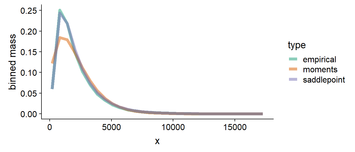
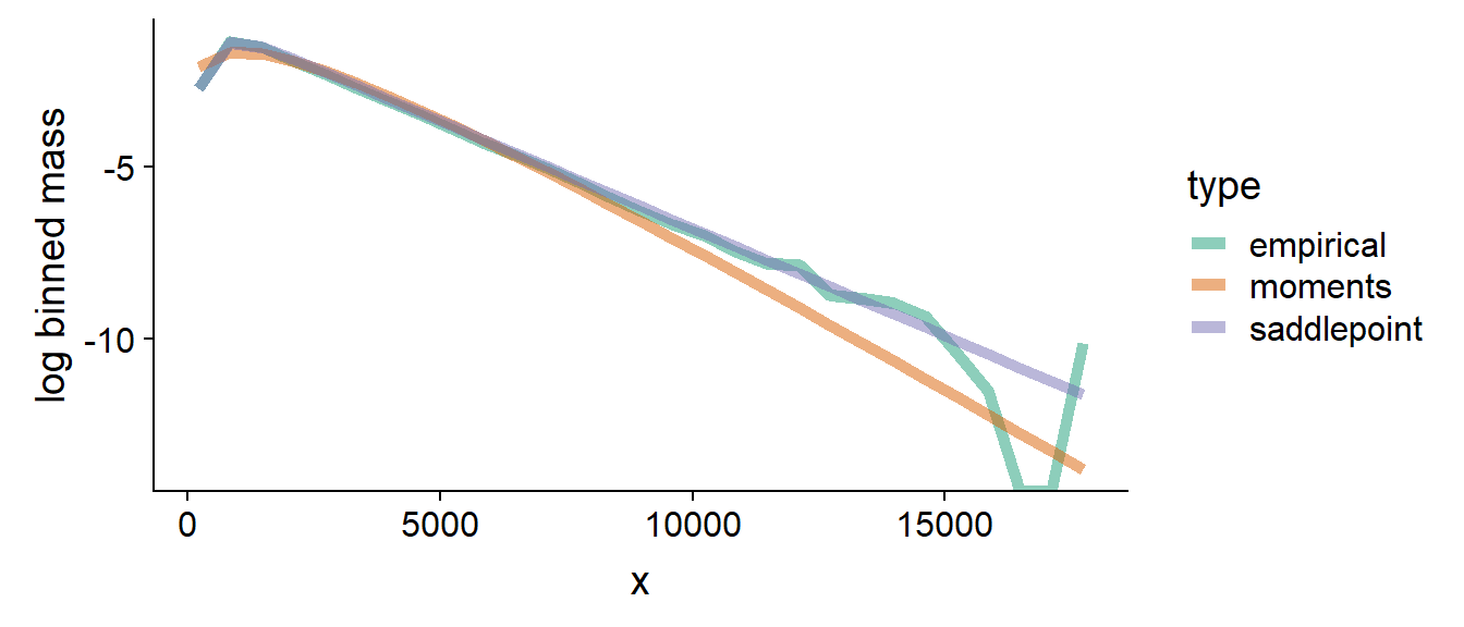
It is visible that the saddlepoint mass tracks the empirical mass very tightly both in the bulk and in the tail (visible better on the log mass) - note that the tail of the empirical log mass is jittery due to low number of samples in the tail.
On the other hand, when we sum a lot of variables which are not very different and/or when \(\phi_i\) are large, the sum becomes normal-ish and both approximation work well - let us for example look at the case when \(\mu = \{50, 100, 1300, 2000 \}\) and \(\phi = \{10, 10, 10, 10 \}\):
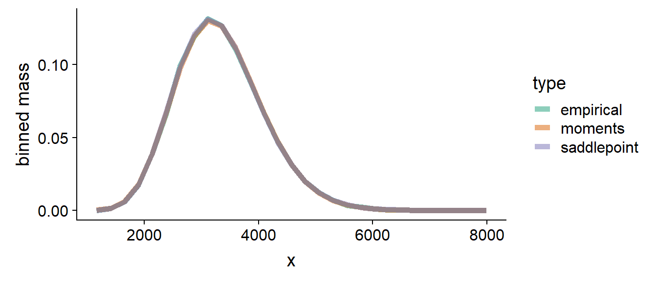
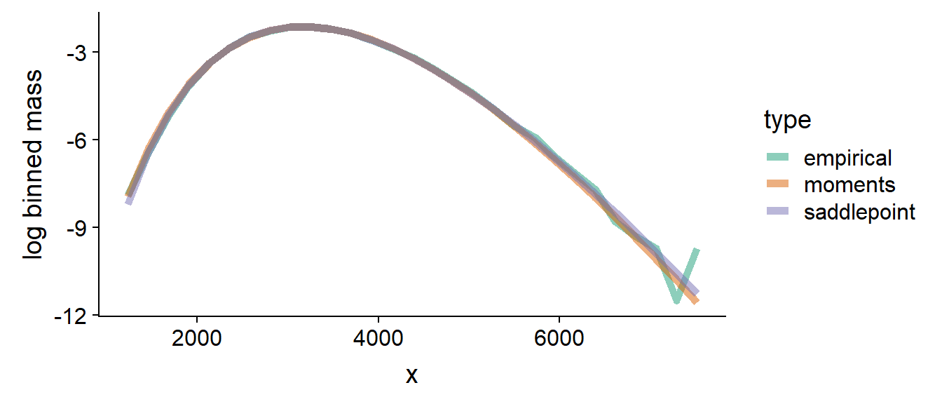
This gives us some intuition where to expect differences.
Evaluating Performance
We evaluate the model using Simulation-based Calibration (SBC). The main idea is that when I generate data exactly the way the model assumes, then for any \(c\) the \(c\%\) posterior interval should contain the true value an unobserved parameter in exactly \(c\%\) of the cases. In other words the quantile in which the true value is found in the posterior distribution should be uniformly distributed. There are some caveats to this, read the paper for details.
I am using my own implementation of SBC which is in my not very well documented, likely-never-on-CRAN package rstanmodeldev. We run 500 simulations for each of the test cases. If you want to see under the hood, the code for this post is available at the GitHub repo of this blog.
The first test case I will use is that I observe the sum of \(G+1\) variables where I know \(\mu_i\) and \(\phi_i\) for \(i \in {1 .. G}\) while \(\mu_{G+1}\) and \(\phi_{G+1}\) is unknown and has to be infered from \(N\) observations of the sum.
In all cases, both observed and unobserved \(\phi_i\) are drawn following the advice of Dan simpson, i.e.:
\[ \phi_{raw} \sim HalfN(0, 1) \\ \phi = \frac{1}{\sqrt{\phi_{raw}}} \]
This is how the model looks-like in Stan ( test_sum_nb.stan ):
#include /sum_nb_functions.stan

data {
  int<lower=1> N;
  int<lower=0> sums[N];
  int<lower=1> G;
  vector[G] mus;
  vector[G] phis;

  //0 - saddlepoint, 1 - method of moments
  int<lower = 0, upper = 1> method;
  real mu_prior_mean;
  real<lower = 0> mu_prior_sd;

}

transformed data {
  real dummy_x_r[0];
}

parameters {
  real log_extra_mu_raw;
  real<lower=0> extra_phi_raw;
}

transformed parameters {
  real<lower=0> extra_mu = exp(log_extra_mu_raw * mu_prior_sd + mu_prior_mean);
  real<lower=0> extra_phi =  inv(sqrt(extra_phi_raw));
}

model {
  vector[G + 1] all_mus = append_row(mus, to_vector({extra_mu}));
  vector[G + 1] all_phis = append_row(phis, to_vector({extra_phi}));

  if(method == 0) {
    sums ~ neg_binomial_sum_saddlepoint_lpmf(all_mus, all_phis, dummy_x_r);
  } else {
    sums ~ neg_binomial_sum_moments_lpmf(all_mus, all_phis);
  }

  log_extra_mu_raw ~ normal(0, 1);
  extra_phi_raw ~ normal(0,1);
}
Most notably, the way the sum of NBs is implemented is given as data. The sum_nb_functions.stan include contains the functions shown above.
And this is an R method to generate simulated data - this is a function that given parameters of the observed data gives a function that on each call generates both true and observed data in a format that matches the Stan model:
generator <- function(G, N, method = "saddlepoint", observed_mean_mus, observed_sd_mus, mu_prior_mean, mu_prior_sd) {
  if(method == "saddlepoint") {
    method_id = 0
  } else if (method == "moments") {
    method_id = 1
  } else {
    stop("Invalid method")
  }

  function() {
    all_mus <- rlnorm(G + 1, observed_mean_mus, observed_sd_mus)
    all_mus[G + 1] <- rlnorm(1, mu_prior_mean, mu_prior_sd)
    all_phis <- 1 / sqrt(abs(rnorm(G + 1)))
    sums <- array(-1, N)
    for(n in 1:N) {
      sums[n] <- sum(rnbinom(G + 1, mu = all_mus, size = all_phis))
    }
    list(
      observed = list(
        N = N,
        sums = sums,
        G = G,
        method = method_id,
        mus = array(all_mus[1:G], G),
        phis = array(all_phis[1:G], G),
        mu_prior_mean = mu_prior_mean,
        mu_prior_sd = mu_prior_sd
      ),
      true = list(
        extra_mu = all_mus[G+1],
        extra_phi = all_phis[G+1]
      )
    )
  }
}
Sum of Two NBs
Here we test a sum of two NBs - the means of both observed and unobserved NB are chosen randomly from LogNormal(5,3) We observe 10 sums in each run.
Saddlepoint
First, let’s look at diagnostics for the saddlepoint approximation:
| has_divergence | has_treedepth | has_low_bfmi | median_total_time | low_neff | high_Rhat |
|---|---|---|---|---|---|
| 0.04 | 0.004 | 0 | 50.0525 | 0 | 0 |
All the columns except for median_total_time represent proportion of fits that have a problem with divergences/treedepth/lowe n_eff etc. We see that some small number of runs ended with divergencies. This is not great, but we will ingore it for now. The n_eff and Rhat diagnostics are okay. We also note that the model is quite slow - 50 seconds for just 10 observations is high.
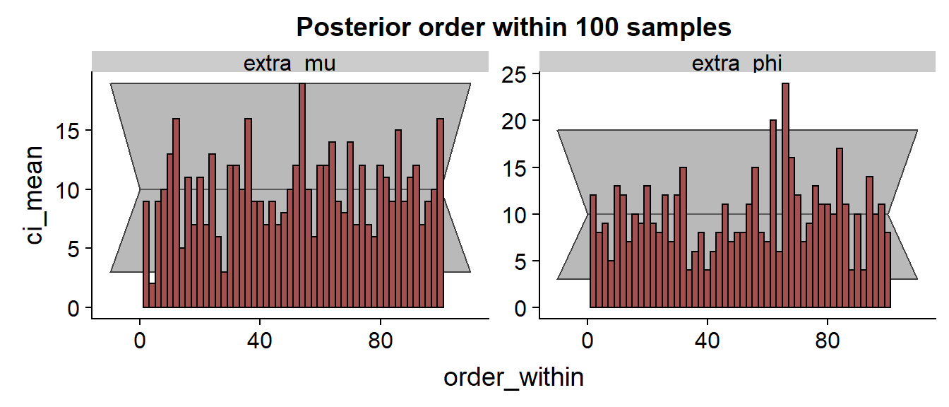
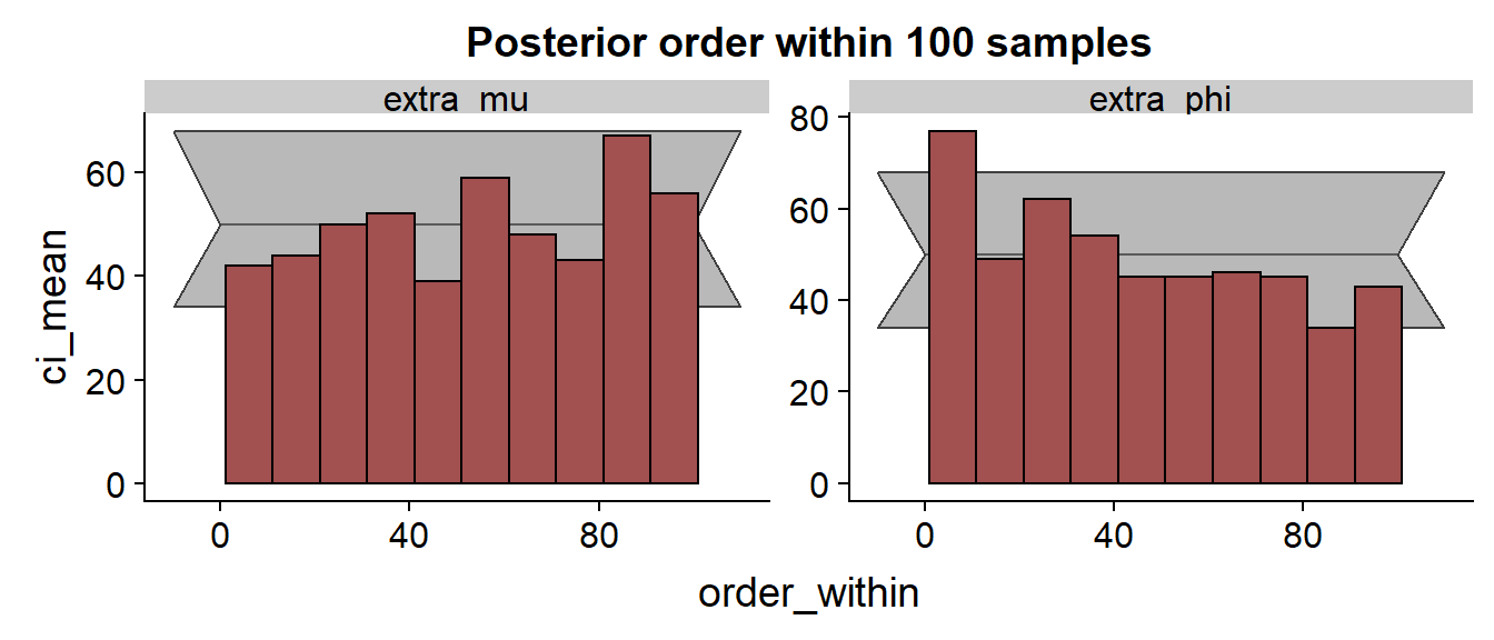
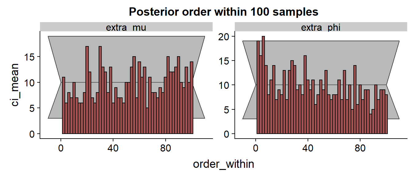
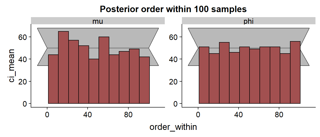
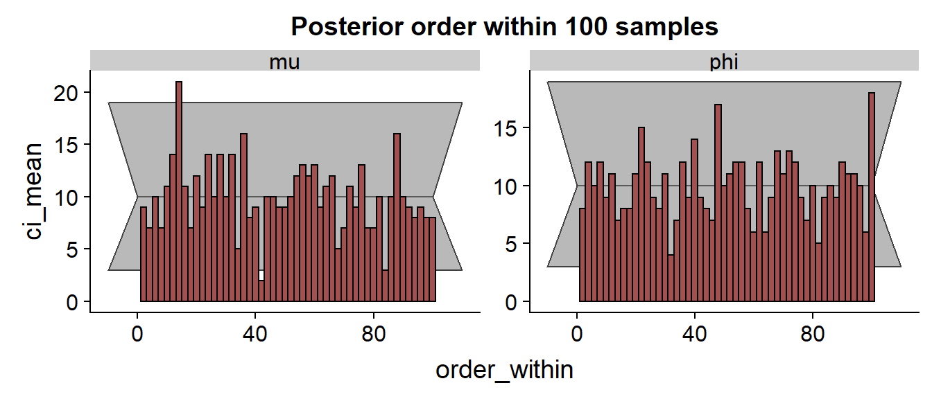
Let’s look at the SBC histogram at two resolutions:
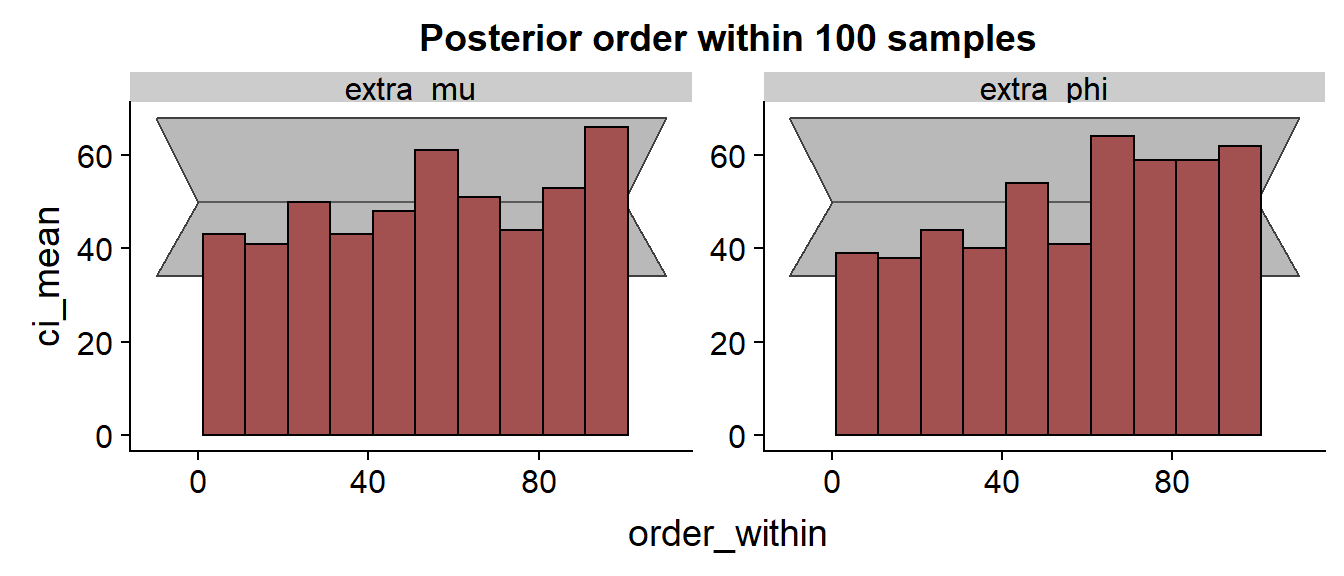
Here we would like to see a uniform distribution. The gray area is a rough 99% confidence interval, so very few bars should actually be outside this. While the histogram for \(\mu_{G+1}\) looks OK, the consistent trend and several outliers for \(\phi_{G+1}\) indicates that the approximation has some problems and consistently underestimates the true value.
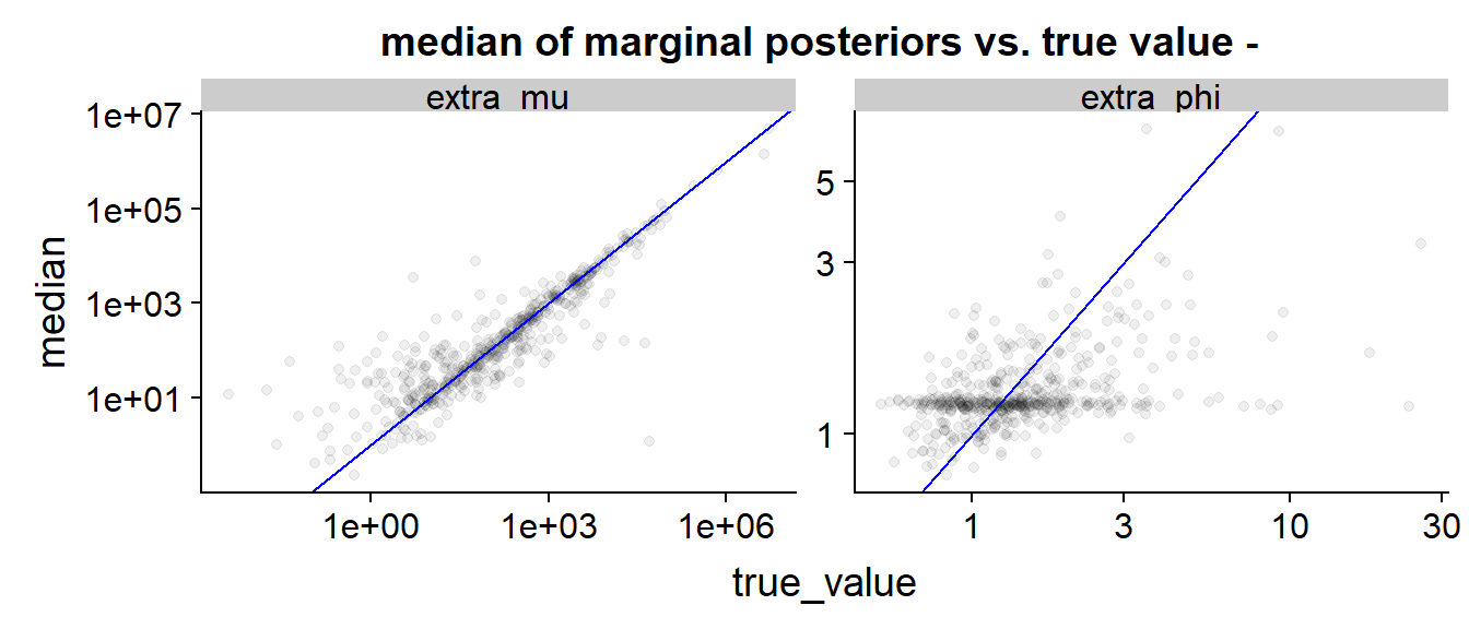
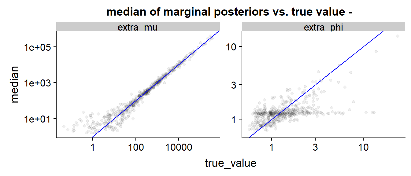
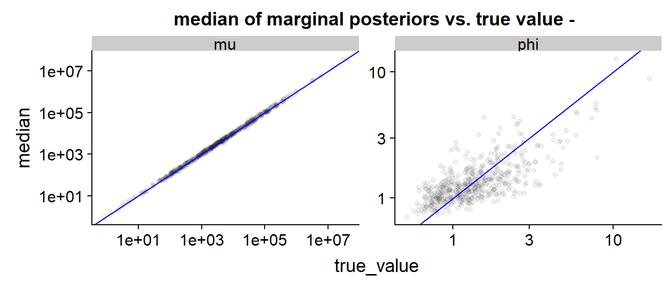
Finally we can look at a scatter plot of true value vs. posterior median:
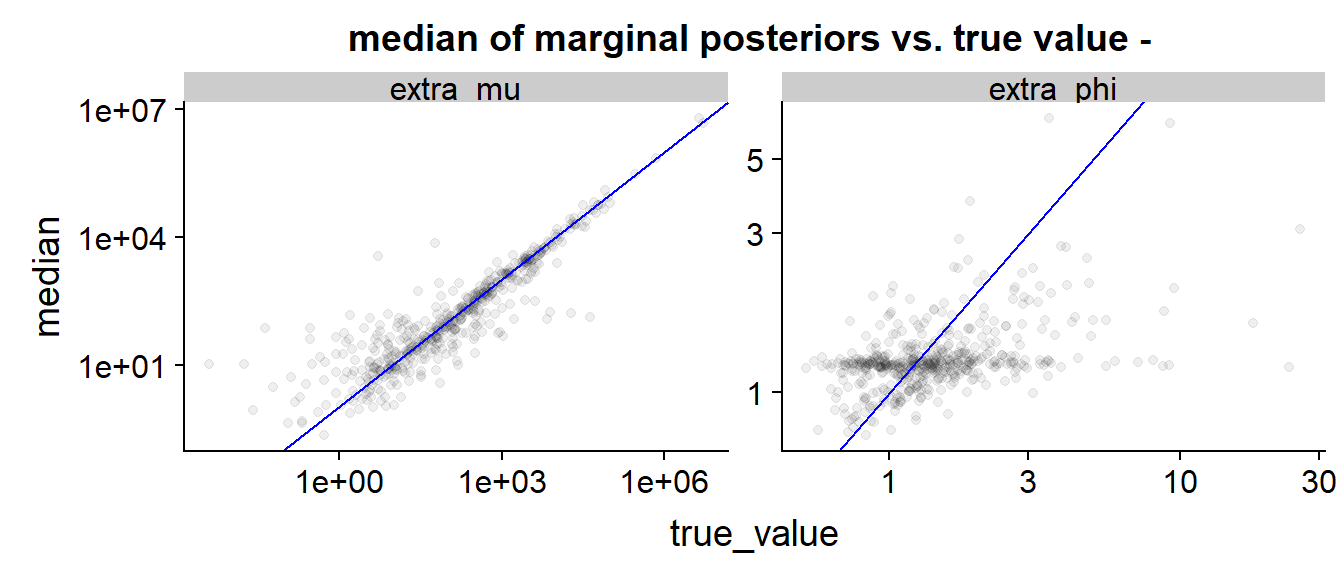
The blue line indicates perfect match (true value = posterior median) As in the above plot, we see that \(\mu_{G+1}\) is inferred quite precisely, especially for larger true values, while the results for \(\phi_{G+1}\) are diffuse, often dominated by the priors (the prior density peaks at around 1.7) and have a slight tendency to be below the perfect prediction line. We also see that low true values of \(\mu_{G+1}\) tend to be overestimated - this is not unexpected as when the observed \(\mu\) is large and unobserved small it is hard to infer it’s exact value and the posterior is largely influenced by prior (which has large mean).
Moments
We can now do the same for the method of moments approximation, starting with the diagnostics:
| has_divergence | has_treedepth | has_low_bfmi | median_total_time | low_neff | high_Rhat |
|---|---|---|---|---|---|
| 0.02 | 0 | 0 | 0.6775 | 0.016 | 0.016 |
We see some small number of divergences and low n_eff and high Rhat (which go usually hand in hand). This is comparable to the saddlepoint case.
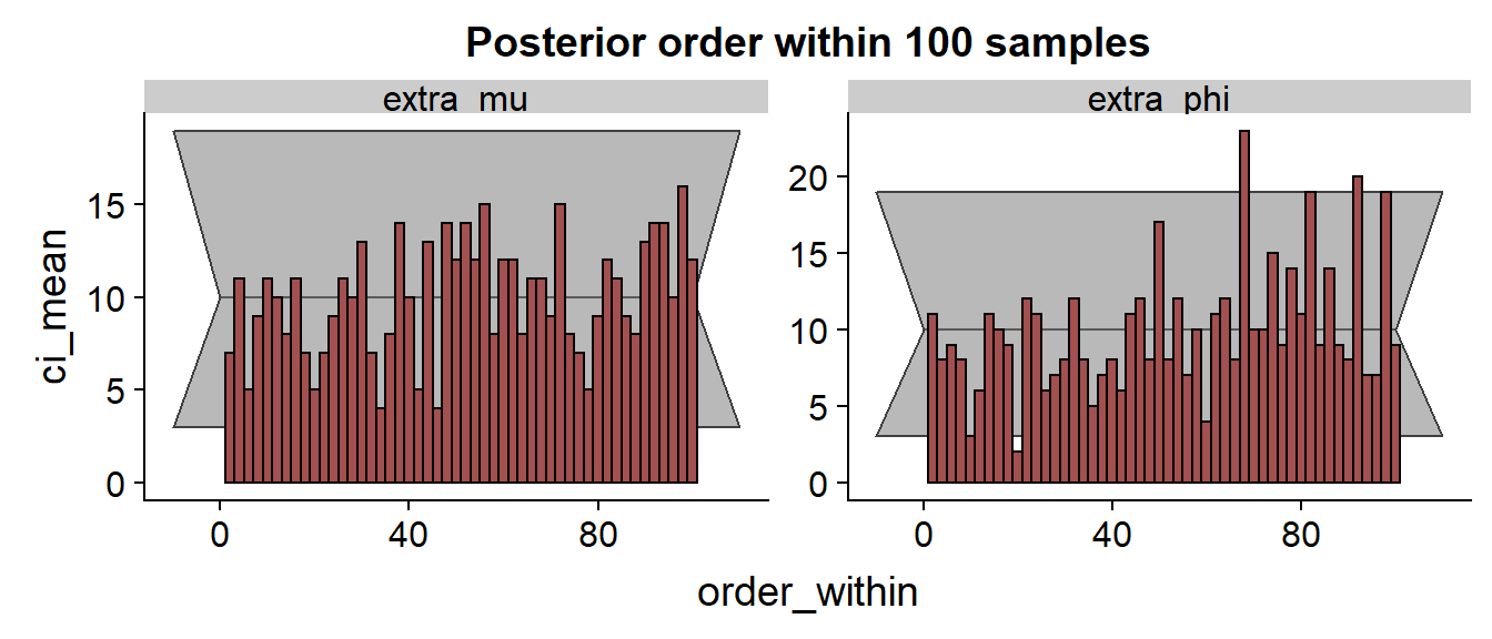
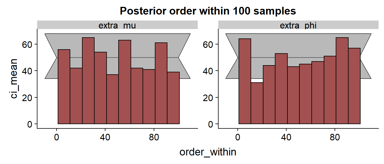
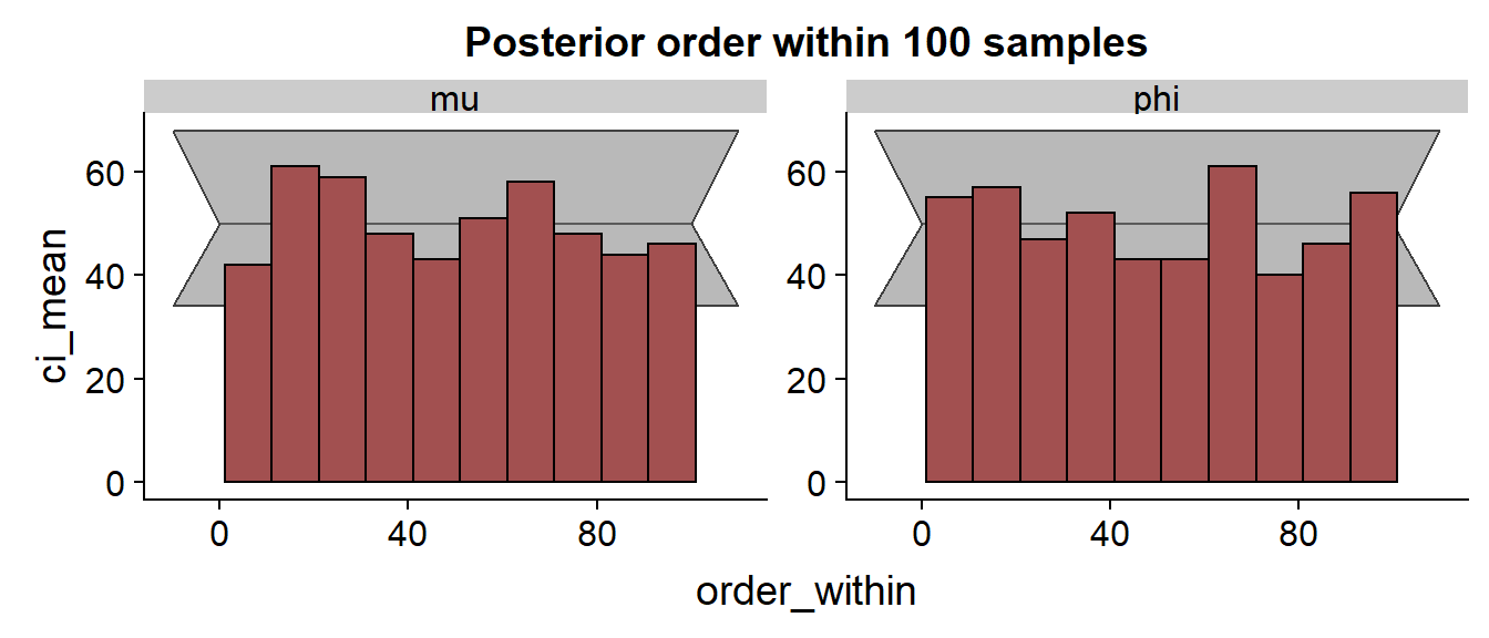
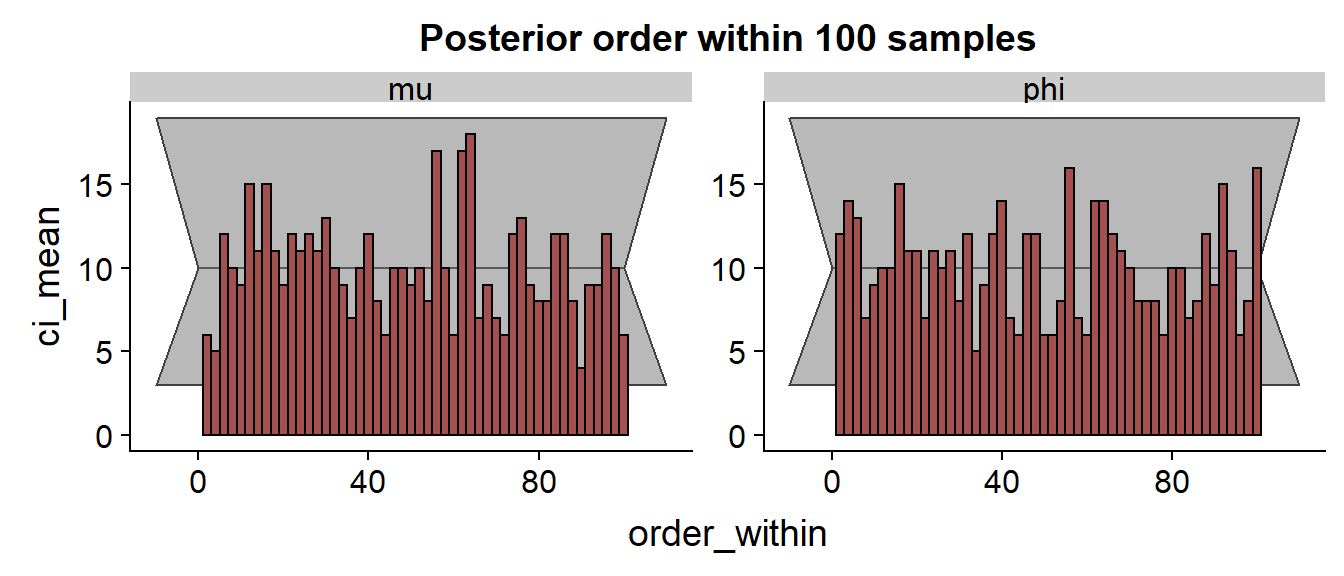
The histogram:
The histrograms look very slightly worse than the saddlepoint approximation - although there is no consistent trend, more bars are outside the confidence interval or close to the border, indicating some issues, although I honestly don’t really understand what is going on.
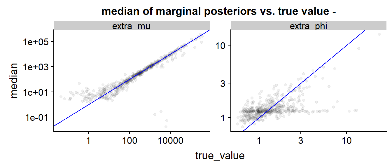
And the scatterplot, which looks quite similar to the saddlepoint version:
Sum of 21 NBs
Further, we can check the case where there are 20 known variables with low means and one NB is unknown with a large mean - we want the unobserved mean to have notable influence on the total outcome, hence we choose it to be larger. In particular, the observed means are drawn from LogNormal(2,1) and the mean to be inferred is drawn from LogNormal(5,3)
Saddlepoint
Looking at the statisics, we see only very few divergences, but quite large median time:
| has_divergence | has_treedepth | has_low_bfmi | median_total_time | low_neff | high_Rhat |
|---|---|---|---|---|---|
| 0.002 | 0 | 0 | 212.1805 | 0 | 0 |
The histogram:
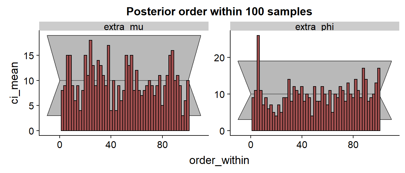
We see that especially for \(\phi_{G+1}\) the results are discouraging with the true value frequently being in the low quantiles of the posterior.
The scatterplot is than quite similar to the previous cases.
Moments
The statistics for moments show short running time but a larger amount of convergence issues:
| has_divergence | has_treedepth | has_low_bfmi | median_total_time | low_neff | high_Rhat |
|---|---|---|---|---|---|
| 0.016 | 0 | 0.008 | 1.0095 | 0.162 | 0.16 |
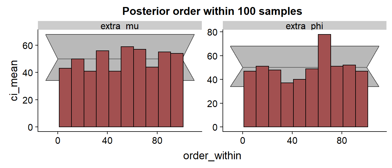
The histograms:
The histograms hint at consistent underestimation of \(\mu_{G+1}\) and overestimation of \(\phi_{G+1}\), problematic especially for \(\phi_{G+1}\).
Once again the scatter is similar, the only interesting feature are the few outliers for \(\mu_{G+1}\) where the true value is large but the posterior median is very small. Those likely correspond to the divergent runs, but they cannot account for the full skew of the SBC histograms - this is more likely caused by the string of underestimated points just below the blue line on the top right.
Sum Defined by Series
The first model is not very useful when G is large, because the posterior gets dominated by the prior. To better test what happens with large G, we instead us a single parameter to define all \(\mu_i\) and \(\phi_i\) as a geometric series, i.e. \(\mu_i = \mu_{base} k^{(i - 1)}\) where \(k\) is known while \(\mu_{base}\) is the unknown parameter, similarly for \(\phi_i\). The Stan code is:
#include /sum_nb_functions.stan

data {
  int<lower=1> N;
  int<lower=0> sums[N];
  int<lower=1> G;

  //0 - saddlepoint, 1 - method of moments
  int<lower = 0, upper = 1> method;

  real mu_prior_mean;
  real<lower = 0> mu_prior_sd;

  real<lower=0> mu_series_coeff;
  real<lower=0> phi_series_coeff;
}

transformed data {
  real dummy_x_r[0];
  vector[G] mu_coeffs;
  vector[G] phi_coeffs;

  mu_coeffs[1] = 1;
  phi_coeffs[1] = 1;
  for(g in 2:G) {
    mu_coeffs[g] = mu_coeffs[g - 1] * mu_series_coeff;
    phi_coeffs[g] = phi_coeffs[g - 1] * phi_series_coeff;
  }
}

parameters {
  real log_mu_raw;
  real<lower=0> phi_raw;
}

transformed parameters {
  real<lower=0> mu = exp(log_mu_raw * mu_prior_sd + mu_prior_mean);
  real<lower=0> phi =  inv(sqrt(phi_raw));
}

model {
  vector[G] all_mus = mu * mu_coeffs;
  vector[G] all_phis = phi * phi_coeffs;

  if(method == 0) {
    sums ~ neg_binomial_sum_saddlepoint_lpmf(all_mus, all_phis, dummy_x_r);
  } else {
    sums ~ neg_binomial_sum_moments_lpmf(all_mus, all_phis);
  }

  log_mu_raw ~ normal(0, 1);
  phi_raw ~ normal(0,1);
}
The R code for simulation is then:
generator_series <- function(G, N, method = "saddlepoint", mu_prior_mean, mu_prior_sd, mu_series_coeff, phi_series_coeff) {
  if(method == "saddlepoint") {
    method_id = 0
  } else if (method == "moments") {
    method_id = 1
  } else {
    stop("Invalid method")
  }

  function() {
    mu <- rlnorm(1, mu_prior_mean, mu_prior_sd)
    phi <- 1 / sqrt(abs(rnorm(1)))
    all_mus <- mu * mu_series_coeff ^ (0:(G - 1))
    all_phis <- phi * phi_series_coeff ^ (0:(G - 1))
    sums <- array(-1, N)
    for(n in 1:N) {
      sums[n] <- sum(rnbinom(G, mu = all_mus, size = all_phis))
    }
    list(
      observed = list(
        N = N,
        sums = sums,
        G = G,
        method = method_id,
        mu_prior_mean = mu_prior_mean,
        mu_prior_sd = mu_prior_sd,
        mu_series_coeff = mu_series_coeff,
        phi_series_coeff = phi_series_coeff
      ),
      true = list(
        mu = mu,
        phi = phi
      )
    )
  }
}
In the following we draw \(\mu_{base}\) from LogNormal(8, 3) and use mu_series_coeff = 0.75 and phi_series_coeff = 0.9.
Saddlepoint
Once again let’s look at the diagnostics for saddlepoint approximation:
| has_divergence | has_treedepth | has_low_bfmi | median_total_time | low_neff | high_Rhat |
|---|---|---|---|---|---|
| 0.054 | 0 | 0 | 155.9085 | 0 | 0 |
We see quite a few divergences, but I didn’t investigate them in detail. The SBC histograms follow:
The histrograms hint at some problems for \(\mu\).

The scatterplot shows that the estimation is quite reasonable for both \(\mu\) and \(\phi\) - definitely better than the previous model, as we got rid of the cases where the data do not identify the true values well.
Moments
The diagnostics and plots for method of moments is:
| has_divergence | has_treedepth | has_low_bfmi | median_total_time | low_neff | high_Rhat |
|---|---|---|---|---|---|
| 0.042 | 0.006 | 0.004 | 0.7445 | 0.004 | 0.002 |
We see a bunch of problems, comparable to the saddlepoint version. Let’s look at the SBC histograms:
And those are surprisingly nice, showing no clear trend or outliers!
The scatterplot is very similar to the saddlepoint case.
Summing up
We see that in the regimes we tested, the saddlepoint approximation for sum of negative binomials provides somewhat better inferences for small number of variables at the cost of much increased computation times. For sums of large number of variables, it may even be worse than the moments method. So it is probably not very practical unless you have few variables you need that extra bit of precision. But it is a neat mathematical trick and of interest on its own. It is also possible that for some low-mean regimes the difference is bigger.
Saddlepoint Approximations for Other Families
If you want to use saddlepoint approximation for other than NB variables, but don’t want to do the math on your own, there are some worked out on the Internet:
- Sum of Gamma variables: Answer on Cross Validated
- Sum of binomials: Liu & Quertermous: Approximating the Sum of Independent Non-Identical Binomial Random Variables
Thanks for reading!